Equipment and Processing - Archive of Side Scan Sonar and Swath Bathymetry Data Collected During USGS Cruise 10CCT01 Offshore of Cat Island, Gulf Islands National Seashore, Mississippi, March 2010

Home | Acronyms | Figures | Navigation | Equipment and Processing |Images | Logs | Metadata | Software

Select the data type:

Side Scan Sonar

Interferometric Swath Bathymetry

Side Scan Sonar

Side Scan Sonar Systems

Side scan sonar is a type of technology used to interpret seabed features, material, and textures from acoustic backscatter response intensity. In this application the instrument (towfish) is towed by a cable aft of the vessel. Once activated, a fan- shaped acoustic pulse is repeatedly emitted downward to the seafloor, perpendicular to a vessel's navigation track, collecting a series of swaths stitched together to create a sonogram, or seafloor image. The towfish can be operated with a range of frequencies; lower frequencies are recorded at a lower resolution but increasing swath range, and higher frequencies record with high resolution at the cost of swath range. High-intensity returns are indications of hard or dense surface material, such as rock or hard-packed sand, whereas low-intensity returns may infer silt or organic material. Intensity images are used in conjunction with physical "grab" samples or cores for the purposed of ground truthing the side scan mosaic.

Side Scan Sonar Acquisition System Components

The side scan sonar components used during Cruise 10CCT01 are as follows:

Klein System 3900 side scan sonar
CodaOctopus Octopus F190 Precision Attitude and Positioning System
OmniSTAR High Performance (HP) correction - 20 cm accuracy

Klein 3900 Side Scan Sonar

Figure 5. Photograph of the Klein 3900 side scan sonar system used for data collection.

Side Scan Sonar Acquisition

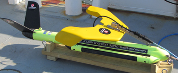
During the 10CCT01 cruise a Klein 3900 dual-frequency side scan sonar system (fig. 5) was towed on the port side of the vessel to collect information about surface sediment material. SSS was acquired and recorded using SonarPro software in an Extended Triton Format (XTF). Differential GPS position from OmniSTAR was recorded by the Octopus F190 Precision Attitude and Positioning System and output in the World Geodetic System of 1984 (WGS84). The towfish altitude varied considerably during the cruise due to the nature of shallow-water surveying operations. Ideally, SSS is flown at a relatively considerable distance from the vessel and other instruments to avoid acoustical interference. Typical sources of acoustical interference are vessel vibrations and other instruments such as sub-bottom profilers and interferometric swath systems that utilize similar frequency ranges. However, in shallow-water surveying the optimal distance is difficult to achieve due to the negative buoyancy of the towfish and the effect of unanticipated isolated shoals.

Side Scan Sonar Processing

The XTF files collected were converted into CARIS data format structure called Sonar Information Processing System (SIPS) for the purpose of editing and sidescan mosaic creation. All horizontal positions were offset relative to the position of the Octopus F190 Precision Attitude and Positioning System antennae.

The first step in SSS data processing was to correct the altitude, or first return. This was achieved by a combination of auto-prediction parameters set and manual boundary digitization of the water column and seafloor.

The second step was application of the beam pattern correction, which was accomplished by sampling a series of beams over homogeneous surface content. The purpose of beam pattern correction is to identify and offset the inherent instrument intensity variance as the across-track range increases. Near nadir the acoustic return is significantly more intense and decreases as across-track range increases. These phenomena result in a false high-intensity value strip along the center line of the SSS swath.

Several other SSS editing tools were applied, including angle-varying gain (AVG) and time-varying gain (TVG) corrections, which were used to further smooth the resulting intensity range artifacts, offering a more consistent along- and across-track image. The despeckle editing tool was also employed to identify and mute isolated pixels having extreme high- or low-intensity values relative to adjacent pixels.

After all the individual side scan line files were examined and edited, Geo-referenced Backscatter Rasters (GeoBars) were created. For this dataset, a resolution of 1 m was chosen. From the series of GeoBars, a sidescan mosaic image was generated as a composite of the GeoBars, which also provides for a continuous image of a single intensity value range for geographic comparison.

In shallow-water surveying (depth less than 15 m for this cruise), a variety of technical phenomena such as multipathing and ping ghosting prove problematic for processing SSS data. Multipathing is the bouncing of the acoustics along the seabed and ocean surface before reaching the extent. This phenomenon is amplified by wave chop, rough weather, and shallow depths. Ghosting is another acoustic anomaly produced by a ping rate which is not slow enough for the transducers to decipher one ping from another. This echoing effect is especially the case in very shallow depths (Hayes and Barclay, 2003).

The side scan mosaic can be viewed on the Images page. Also, the GeoTIFF image can be found in the Data Products folder. Please reference the read-me file for file names and details.

Interferometric Swath Bathymetry

Interferometric Swath Systems

A swath-sounding sonar system is used to measure the depth in a line extending outward from the sonar transducer. As the survey vessel moves along a trackline, the swath transducer sends out sonar signals at a right angles to the trackline and is scanning the seabed to each side of the vessel. It sweeps out an area of depth measurements, referred to as a swath. The word interferometric refers to the technique used to measure soundings. The interferometric technique uses the phase content of the sonar signal to measure the wave front that is returned from the seafloor or other targets such as a seawall.

Interferometric sonar systems require three or more linear arrays of transducer elements, one to transmit acoustic energy and at least two to receive the returning signal (SEA Ltd., 2005). These arrays, also called staves (fig. 6), are housed within the black housing known as the transducer. Depth measurements from interferometric systems are calculated by measuring two factors, the travel time of a sound pulse and the angle at which the pulse returns to the transducer. More generally, when a sound pulse is emitted from the transducer it travels to the seafloor and then travels back to the transducer. The time it takes to do this is the travel time, also referred to as the range. The second measurement is the angle at which the returning sound pulse is received by the transducer. The combination of these pairs calculates a depth value (SEA Ltd., 2005).

Swath System Acquisition Components

The swath system components used during Cruise 10CCT01 are as follows:

SEA Ltd. SWATHplus-H 468-kHz Interferometric System
CodaOctopus Octopus F190 Precision Attitude and Positioning System
OmniSTAR High Performance (HP) correction 20-cm accuracy

Glacier Bay Catamaran and sled mounted swath

Figure 6. Photograph of the Glacier Bay Catamaran and sled-mounted swath transducers used in data collection for Cruise 10CCT01.

Swath System Field Calibration and Acquisition

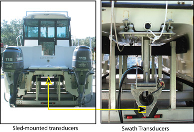
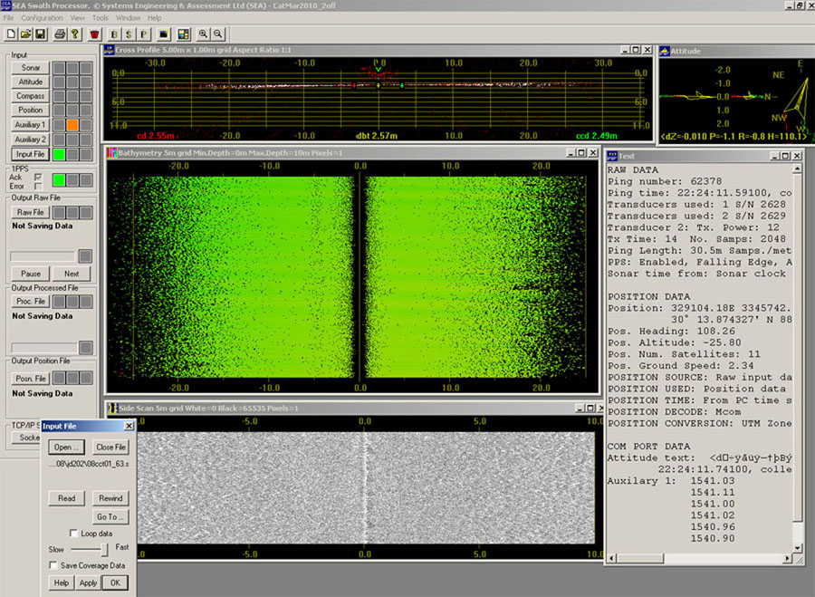
The swath bathymetry was collected using the SEA Ltd. SWATHplus-H Interferometric system (fig. 6) and SEA Swath Processor software version 3.6 (fig. 7). The system must be calibrated before the survey commences. This involves inserting the CodaOctopus Octopus F190 Precision and Attitude Positioning System's sensor and antennae positions and offset values into the program, restarting the program with these correct offsets, and proceeding to calibration maneuvers. The vessel needs to execute some type of motion (circles or figure eights) for approximately 30 minutes during the calibration process. The calibration program allows the sensor to orient itself relative to the vessel and obtain a lock on position which will ensure accurate motion and position data in real time during swath acquisition.

Screen shot of SEA SWATHplus Acquisition and Processing Interface.

Figure 7. Screen shot of SEA SWATHplus Acquisition and Processing Interface.

Calibration of the SEA SWATHplus sonar head involved entering all setup data parameters into a SEA SWATHplus session file (SXS) and then running a roll calibration test also known as a patch test. The roll calibration consisted of seven lines that were 900 m long and spaced 25 m apart to obtain 100 percent overlap coverage. The lines are surveyed in a manner in which the port swath will overlap the previous port swath and the starboard swath will overlap the previous starboard swath. These surveyed lines were then input into SEA Ltd.'s Grid Processor program version 3.07. The Grid Processor has a roll calibration program that runs a series of calculations on the port-to-port swaths and the starboard-to-starboard swaths that produces a roll angle value that reflects the transducer orientation aboard the respective vessel. These final transducer roll angle values for the port and starboard, respectively, were added to their default angle (-30 degrees) within the SXS configuration file prior to processing of bathymetry lines.

During acquisition, the differentially corrected positions supplied from OmniSTAR were recorded by the Octopus F190 and output in the WGS84 datum. Boat position and motion data (roll, pitch, and heave) from the Octopus F190, and swath depth measurements were streamed in real time to a dedicated laptop computer. A Valeport Mini Sound Velocity Sensor (SVS) was attached to the transducer head to supply speed of sound (SOS) measurements simultaneously. The SXS used during setup and calibration was used during survey to record all streaming data into the SEA Swath Processor Raw File (SXR) format and the SEA Swath Processor Coverage File (SXC) format. During the survey, three SOS casts were measured using a Valeport Mini Sound Velocity Probe (SVP) and recorded manually. All data were backed up digitally onto Blu-ray media and terabyte servers.

Swath Bathymetry Processing

SEA Swath Processor

The swath bathymetry was post-processed using SEA SWATHplus version 3.07, an upgrade that was available for this dataset. The SXS files used for acquisition were also used for post-processing, which included all the respective roll calibrations, offsets, and SOS measurements. The SVP casts were entered manually to help correct for SOS and reduce the production of refraction artifacts. The SXR files were replayed through the SEA Swath Processor program to produce SEA Swath Processor Processed Files (SXP), which have been geometrically processed and corrected.

CARIS Processing

The SXP files produced were then edited in CARIS HIPS and SIPS version 7.0, which provided for further manipulation and editing of the swath bathymetry. The SXP files were imported using the CARIS Conversion Wizard, which converts processed data into the Hydrographic Information Processing System (HIPS) format. At this point the swath lines were not tidally corrected and referenced to Mean Low or Lower Water (MLLW). In CARIS, the Load Tide feature was implemented to reference the swath bathymetry measurements to MLLW using a tide zone model and verified tide data from two tide stations: Pascagoula, MS, station ID 8741533 and the Gulfport, MS, station ID 8745557. The tidal zone definition was created and supplied by National Oceanic and Atmospheric Administration (NOAA). All files were then merged to apply all corrections.

After the merge process, each line was filtered and edited using CARIS Swath Editor to remove stray points and reject noisy outer beams. When a line displayed depth consistency along-track, it was possible to use the across-track distance filters to smooth the results. Other filters applied included depth, beam-to-beam slopes, and missing neighbors. In some instances there were SOS refraction artifacts seen in segments of the bathymetry lines; these artifacts looked like a smile or a frown. If this occurred the CARIS Refraction Editor, a component within the Swath Editor, could be used to manually apply an SOS value to reduce the effects in the portions of lines where sound velocity casts were not sufficiently correcting the data. The files were remerged after the editing process. When the files were clean of errant values, a 10-meter Bathymetry Based on Statistical Error (BASE) surface was created. The 10-m BASE surface represents a depth value averaged from points every 10 m along the swath transect. The BASE surface was further reviewed for major areas that may have been missed or that appeared to be outstanding and questionable relative to their surrounding data. If found, these areas were edited accordingly, remerged, and the BASE surface recomputed. When the BASE surface was considered clean, further review of minor editing and data cleaning was followed using the CARIS Subset Editor. Subset Editor edits a portion of the surface and only recomputes the selected area; this step allows for minor adjustments if necessary. To enhance the definition of the Gulfport Ship Channel, four swath bathymetry lines from USGS Cruise 10CCT02 taken within the channel were processed accordingly and incorporated into the BASE surface for 10CCT01. Information and FACS forms for 10CCT02 are located at http://coastal.er.USGS.gov/field-activity-schedule/. When the BASE surface was considered complete, the BASE surface x, y, z values were exported in ASCII format.

The x, y, z, ASCII file was imported into ESRI’s ArcMap version 9.3.1 and gridded using the Geostatistical Analyst Tool's radial basis functions. This tool allowed adjustment to the interpolation parameters with regard to real-data spatial resolution and orientation. The interpolation parameters once set are then used by the tool for predicting values. This method provided more of an accurate and less biased representation of the dataset as a whole. A cross-validation report can be generated when using the radial basis function. This helps the user understand how well the model will predict data values at unknown locations. In general the cross validation takes one point and predicts that point's position using the surrounding data values. The result is a predicted value. This predicted value is compared against the actual value of that data point and general statistics computed. The ESRI cross-validation report for the swath bathymetry 50-m grid is listed below.

	Measured	Predicted	Error
Points	105,892	105,892	105,892
Minimum	-12.96	-12.75	-1.98
Maximum	-0.90	-0.93	+1.69
Mean	-5.28	-5.28	0.001
Standard Deviation	2.08	2.07	0.093

The swath and side scan sonar surfaces can be viewed on the Images page. Also, the files can be found in the Data Products folder. Please reference the read-me file for file names and details.