Potential Effects of Individual Sewage Disposal System Density on Ground-Water Quality in the Fractured-Rock Aquifer in the Vicinity of Bailey, Park County, Colorado, 2001-2002
Fact Sheet 2004–3009
By Daniel L. Brendle
Available from the U.S. Geological Survey,
Branch of Information Services, Box 25286,
Denver Federal Center, Denver, CO 80225, USGS Fact Sheet 2004-3009.
(Requires Adobe Acrobat Reader)
| Introduction
Park County, about 30 miles southwest of Denver (fig. 1), is one of the fastest growing counties in Colorado. With the increasing population and development in rural areas comes an increase in demand for water resources, the number of individual sewage disposal systems (ISDS), and the potential to affect the ground-water quality. Health department officials, planners, and County Commissioners in Park County are interested in obtaining information regarding water quality in aquifers that serve the residents of the county. In 2000, the U.S. Geological Survey (USGS), in cooperation with Park County, began a study to determine the effects of residential development and the concurrent increase in ISDSs and the density of ISDSs on ground-water quality in the various aquifers in Park County that supply water to domestic wells. This report provides a preliminary assessment of water-quality data collected in 2001 from domestic wells completed in the fractured-rock aquifer in the vicinity of Bailey in northeastern Park County (fig. 1). Water samples were collected from 57 domestic wells during 2001, once in July and once in September. Samples were analyzed for chemicals and bacteria that might indicate whether ISDS effluent has caused degradation of ground-water quality. This report also describes the preliminary results of five water samples collected in October 2002 for tritium analysis. The granitic and metamorphic (crystalline) rocks (Tweto, 1979) in the Bailey area contain ground water in fractures and form the principal aquifer supplying domestic wells. Reported well yields for wells drilled into the fractured crystalline rock range from less than 1 gallon per minute (gal/min) to 60 gal/min. The variability in well yields depends on many things, including the number of fractures intercepted by a well, the degree of openness of those fractures, and the length of the open interval of the well (fig. 2). Well yields for sampled wells ranged from about 0.5 to 25.5 gal/min. Depths for wells chosen for sampling ranged from 85 to 752 feet. The well yields and depths for wells sampled are representative of most of the wells drilled in the crystalline-rock aquifer in the vicinity of Bailey (Colorado Division of Water Resources, 2000). |
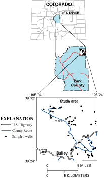 Figure 1. Location of study area. |
|
|
The amount of time it takes for water to recharge the aquifer and reach the wells varies with the openness and connectedness of the fractures, the distance from the recharge point to the open interval of a well, and the rate of water flow in the fractures. Because the rate of recharge and flow in the vicinity of each well can vary, it is not known whether ISDS effluent can reach the ground water before chemical and biological contaminants are removed from the effluent or reduced in concentration. This study was designed to assess whether contamination of ground water has occurred and to obtain information that might help determine the length of time it takes for ISDS effluent to recharge the aquifer. The size of the lots in each development, and thus the closeness of neighboring wells and ISDSs, varies. Each residence has its own ISDS. House densities range from several houses per acre to a single house on many acres. As houses are built closer to each other and as ISDS density increases, there could be a greater potential for degradation of ground-water quality. Potential Effects of Individual Sewage Disposal System Effluent on Ground-Water Quality Geochemical and physical processes occur in the subsoil—unsaturated zone above the water table and the saturated zone below the water table (fig. 2)—that can reduce the concentrations of chemical and biological constituents in ISDS effluent. For a properly functioning ISDS, most of the potential contaminants in the effluent are removed by filtration or oxidation in the unsaturated zone below the leach field and above the water table (Wilhelm and others, 1994). When effluent reaches the unsaturated zone above the water table, it flows through the pores between the particles, such as sand and gravel from the weathered crystalline rock, that make up the subsoil. Large particles and bacteria in the effluent can be filtered by the subsoil, leaving mostly dissolved compounds in the effluent. As the effluent flows through the subsoil and is exposed to oxygen, ammonia is oxidized to form nitrate (nitrate plus nitrite, as nitrogen). When nitrate reaches the water table, and if dissolved organic carbon (DOC) is present and dissolved oxygen is absent, the nitrate and DOC may be consumed by denitrifying bacteria to produce nitrogen and carbon dioxide gasses. Thus, the concentration of nitrate increases beyond the leach field but then decreases as it travels through the saturated zone (Robertson and others, 1989). |
||
| Caffeine and other organic chemicals can be degraded to other compounds by bacteria in the saturated zone in the vicinity of the leach field from which the compounds originated. However, organic chemicals can persist in ground water if degrading bacteria are not present. Biological constituents in ISDS effluent that can cause disease (pathogenic organisms) include bacteria and viruses. These microorganisms have different survival rates and transport properties in the saturated and unsaturated zones below a leach field. For example, Escherichia coli (E. coli) can potentially survive for several weeks in the subsurface if conditions are favorable (Matthess and Pekdeger, 1981). It is not known whether E. coli can survive long enough in a fractured-rock setting to be transported to the water table and eventually to wells. Total coliform and E. coli bacteria can be removed from ISDS effluent by filtration as the effluent flows through the unsaturated zone (Viraraghavan and Warnock, 1976). However, if the water table lies closer to the land surface, the unsaturated zone is thinner and more of the bacteria in the effluent can potentially reach the ground water (Canter and Knox, 1985). |
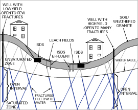 Figure 2. Diagram showing the relation of Individual Sewage Disposal System, domestic wells, and the water table in a fractured-rock ground-water system. |
|
| Indicators of Contamination
to the Ground Water
Samples collected from wells were analyzed for chemicals and bacteria that can originate from an ISDS. Many of these chemicals and bacteria can enter the ground water through natural processes, but if they are observed in elevated concentrations it can indicate degraded ground-water quality. Chloride, nitrate, nitrite, ammonia, and boron can all occur naturally in ground water. These chemicals usually do not occur naturally at elevated concentrations because these chemicals come from dispersed sources, such as waste from wild animals, decomposition of forest material, deposition from the atmosphere, or from weathering of rocks. An ISDS can provide a focused source of these chemicals if its leach field pipe is too close to the water table or if the infiltration rate and ground-water flow velocity are too rapid to allow for proper geochemical or physical treatment of the ISDS effluent. Products that are used in households, such as soaps containing boron, dietary salt containing chloride, caffeine, pesticides, perfumes, or human waste containing nitrate, nitrite, and ammonia, can enter the ground-water system as a more concentrated effluent from an ISDS. Total coliform and E. coli bacteria can originate from humans and other warm-blooded animals. Sampling Plan Design and Methods The plan for collecting ground-water samples was
designed to allow an evaluation of whether the density of development
and thus the proximity of wells and ISDSs (ISDS density) is a factor
in potential degradation of ground-water quality. Private wells
were used as a surrogate for locating ISDSs because those lots having
a well and a house also have an ISDS, and records for wells are
more easily accessible than records of ISDSs. Thus, well density
is equivalent to ISDS density for the purposes of this analysis.
Wells listed in Colorado public well records (Colorado Division
of Water Resources, 2000) were divided into four categories based
on the number of wells per acre: more than one well per acre (high-density);
one well in 3 acres (medium-density); one well in 5 or more acres
(low-density); and background wells (wells that were not expected
to be influenced by other wells and ISDSs) (background) (table 1).
Candidate wells were classified into one of the three density categories by plotting their locations on a map and overlaying a grid on the map in GIS. Each of the overlay grids was made of cells that represent areas of 1 acre, 3 acres, or 5 acres. Well density was confirmed by observations made in the field. When the list of candidate wells was exhausted, additional wells needed to complete the sample size for each density category were chosen based on field observations. Background wells were chosen using the criterion that the wells were located such that the water pumped by the wells was not expected to be influenced by ISDSs or other human activities. Wells were sampled for chemicals and bacteria that can originate from septic systems and can be used as indicators of ground-water-quality degradation, including boron, chloride, fluoride, sulfate, nitrate, ammonia, phosphorus, total coliform and E. coli bacteria, and 67 organic chemicals that can only originate from households, such as caffeine, perfumes, pharmaceuticals, and the metabolites of organic chemicals (Kolpin and others, 2002). Samples were collected from a faucet in the plumbing system of each house and the water was pumped by the existing pump in each of the wells. Standard USGS protocols for the collection of water-quality samples were followed (Wilde and others, 1998). Measurements of the physical characteristics of water, such as pH, dissolved oxygen, and specific conductance also were made. Additionally, most wells were sampled twice, once each in July and September, to determine whether there were detectable variations in water quality with time (table 1). Quality-control samples collected in the field included eight blank and five replicate samples. Results indicate that field procedures did not contaminate the environmental samples. Data used in this analysis can be obtained on the Web at this URL: https://waterdata.usgs.gov/co/nwis/qwdata (search for Park County and the date range when the samples were collected). Water samples were analyzed at the USGS National Water Quality Laboratory in Denver, Colorado, using methods described in Fishman (1993) for inorganic chemicals and in Zaugg and others (2002) for organic chemicals. Methods used to compare data The results of analysis of the samples were grouped by the density categories and the month the well was sampled. The concentrations of chemicals and bacteria in the samples were then compared to assess whether differences existed between the density categories and the month the sample was collected. Sample results were compared by using boxplots and testing for differences between the groupings of data by using the Wilcoxon rank-sum test (Helsel and Hirsch, 1992). Boxplots provide a visual comparison of the variability between
data from different density categories and from different months.
An example of a boxplot is shown below: The Wilcoxon rank-sum test is used to determine whether a statistical difference exists between two data sets. All possible combinations of two data sets for a particular chemical for all density categories and months were evaluated using the rank-sum test. Differences between data sets were determined to be significant when the significance level (p-value) was 0.05 or smaller. A p-value of 0.05 means that it can be said with 95-percent confidence that two data sets being compared are different. As the p-value increases, the level of confidence that two data sets are different decreases. Potential Effects of Individual Sewage Disposal System Density on Ground-Water Quality Four of the samples collected in July and four collected in September contained bacteria; only one well had detections of bacteria in both months. Detections of bacteria indicate contamination of the ground water, but not necessarily from an ISDS. Bacteria were present in samples from wells in the low-, medium-, and high-density categories. Detections of bacteria did not appear to be correlated with ISDS density. Additionally, concentrations of the other chemicals associated with ISDSs in these samples were not above expected background concentrations. Samples from four wells in the low-density and background categories contained organic chemicals that can originate only from an ISDS. One of the 67 organic chemicals was detected in each of 3 wells, and 2 of the chemicals were detected in 1 well. The detections of organic chemicals might be due to ISDS contamination, but concentrations of the other chemicals in the samples were not elevated above expected background concentrations. A comparison was made to determine whether there was a correlation between concentrations of the various chemicals and the depths or yields of wells. This comparison indicated that the concentrations of several chemicals were inversely related to the depths or yields of wells (as yield or depth increases, concentrations decrease), but the correlations were not very strong. Data from all wells were plotted on boxplots, and the Wilcoxon rank-sum test was used to identify statistically significant differences between months for a selected density category and chemical, or between density categories for a particular month and chemical. Most of the tests indicated no significant differences. None of the tests indicated a significant difference between July and September for a particular density category and chemical. The boxplots are shown only for those chemicals that had at least one comparison that was statistically significant: nitrate, chloride, and boron. The boxplots indicated the lowest concentration for a particular chemical was nearly the same for all density categories. These plots also show that the difference between the highest and lowest concentrations for a particular chemical was greatest for the high-density category and smallest for the background category. | ||
| Significant differences as determined by the Wilcoxon rank-sum test for the nitrate data were found (fig. 3): between the high- and low-density categories for July data; and between the high- and low-density categories and the high-density and background categories for September data. Figure 3 indicates that the median nitrate concentration in the high-density category was about 35 percent greater than the median for the medium-density category, about 75 percent greater than the median for the low-density category, and about 64 percent greater than the median for the background category. These comparisons and the boxplots indicate nitrate concentrations tended to be higher in the high- and medium-density categories than in the low-density or background categories. The comparisons also indicate a higher probability of transport of nitrate to the ground water in areas with a higher density of houses and their associated ISDSs. However, in the high-density category only 7 percent (two samples) of the samples had nitrate concentrations greater than the U.S. Environmental Protection Agency (USEPA) primary drinking-water standard of 10 milligrams per liter (mg/L), and 17 percent (five samples) had nitrate concentrations from 9 to 10 mg/L. The maximum nitrate concentration was 25.7 mg/L from a well in the high-density category. None of the nitrate samples from the low-density category exceeded the USEPA standard for nitrate; the maximum nitrate concentration in this density category was 9.2 mg/L. These data indicate a propensity for elevated nitrate concentrations in areas where ISDS densities are more than one ISDS per 5 acres, but the data also indicate that elevated nitrate also occurs in the low-density and background categories. |
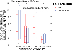
Figure 3. Boxplot of nitrate data for all density categories and both months when samples were collected. See table 1 for the number of samples in each category. |
|
| Significant differences as determined by the Wilcoxon rank-sum test for the chloride data were found (fig. 4): between the high- and low-density categories and the high-density and background categories for July data; and between the high- and medium-density categories, the high- and low-density categories, and the high-density and background categories for September data. Figure 4 indicates that the median chloride concentration in the high-density category was about 26 percent greater than the median for the medium-density category, about 65 percent greater than the median for the low-density category, and about 69 percent greater than the median for the background category. These comparisons and the boxplots indicate chloride concentrations tended to be higher in the high- and medium-density categories than in the low-density or background categories. The comparisons also indicate that there may be a higher probability of transport of chloride to the ground water in areas with higher density of houses and their associated ISDSs. However, in the high-density category only 7 percent (two samples) of the samples had chloride concentrations greater than the USEPA secondary drinking-water standard of 250 mg/L. None of the chloride samples from the low-density category exceeded the USEPA standard for chloride; the maximum chloride concentration in this density category was 51.3 mg/L. The maximum chloride concentration was 886 mg/L for a sample from the high-density category. | 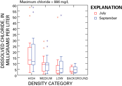
Figure 4. Boxplot of chloride data for all density categories and both months when samples were collected. See table 1 for the number of samples in each category. |
|
| Significant differences as determined by the Wilcoxon rank-sum test for the boron data were found (fig. 5) only between the high- and low-density categories for September 2001 data. Figure 5 indicates that the median boron concentration in the high-density category was about 24 percent greater than the median for the medium-density category and about 39 percent greater than the medians for the low-density and background categories. The maximum boron concentration was 144 micrograms per liter (µg/L) for a sample from the high-density category. |
||
| Five tritium samples were collected between October 11–15, 2002, to attempt to determine an approximate age, or time since recharge, of the ground water pumped by wells. Tritium is used as an age-dating tracer because it was produced in relatively high concentrations as a result of atmospheric nuclear bomb testing beginning in 1954 (Kendall and others, 1998). Concentrations of tritium do not definitively yield the age of the water in a sample but must be used with other age-dating chemicals to refine the age estimate. Ground water having a certain tritium concentration is likely to contain a mixture of waters of different ages that exhibit a composite age based on the proportions of different-age waters contributing to a sample. Concentrations of tritium in the samples ranged from 15 to 38 picocuries per liter (tritium data can be obtained on the Web at URL http://waterdata.usgs.gov/co/nwis/qwdata (search for Park County and date range October 11-15, 2002)). Concentrations greater than 10 picocuries/liter indicate that recharge to the ground-water system occurred after 1954 (Kendall and others, 1998). Additional data analysis of the age-dating chemicals is needed to evaluate the age of ground water and the vulnerability of the ground water to contamination. |
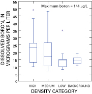
Figure 5. Boxplot of boron data for all density categories for samples collected in September. See table 1 for the number of samples in each category. |
|
| References Cited Canter, L.W., and Knox, R.C., 1985, Septic tank system effects on ground water quality: Chelsea, Mich., Lewis Publishers, 336 p. Colorado Division of Water Resources, 2000, public well records available from the Division of Water Resources Records Section, Denver, Colorado. Fishman, M.J., ed., 1993, Methods of analysis by the U.S. Geological Survey National Water Quality Laboratory—Determination of inorganic and organic constituents in water and fluvial sediments: U.S. Geological Survey Open-File Report 93–125, 217 p. Helsel, D.R., and Hirsch, R.M., 1992, Statistical methods in water resources: New York, Elsevier Science Publishing Company, Inc., 522 p., 1 diskette. Kendall, C., and McDonnell, J.J., eds., 1998, Isotope tracers in catchment hydrology: New York, Elsevier Science Publishing Company, Inc., 839 p. Kolpin, D.W., Furlong, E.T., Meyer, M.T., Thurman, E.M., Zaugg, S.D., Barber, L.B., and Buxton, H.T., 2002, Pharmaceuticals, hormones, and other organic wastewater compounds in U.S. streams, 1999–2000-A national reconnaissance: Environmental Science and Technology, v. 36, no. 6, p. 1202–1211. Matthess, G., and Pekdeger, A., 1981, Survival and transport of pathogenic bacteria and viruses in ground water, in Proceedings, First International Conference on Ground-Water-Quality Research, Houston, Texas, John Wiley and Sons, N.Y., p. 472–482 Robertson, W.D., Sudicky, E.A., Cherry, J.A., Rappaport, R.A., and Shimp, R.J., 1989, in Kobus, H.E., and Kinzelbach, W., eds., Impact of a domestic septic system on an unconfined sand aquifer: Proceedings of the international symposium on contaminant transport in ground water, Stuttgart, Federal Republic of Germany, April 4–6, 1989, v. 3, p. 105–112. Tweto, Ogden, comp., 1979, Geologic map of Colorado: U.S. Geological Survey State Geologic Map, scale 1:500,000 (reprinted). Viraraghavan, T., and Warnock, R.G., 1976, Groundwater quality adjacent to a septic tank system: Journal of the American Water Works Association, v. 68, no. 11, part 1, p. 611–614. Wilde, F.D., Radke, D.B., Gibs, J., and Iwatsubo, R.T., 1998, National field manual for the collection of water-quality data: U.S. Geological Survey Techniques of Water-Resources Investigations, book 9, chap. A1–A9. Wilhelm, S.R., Schiff, S.L., and Cherry, J.A., 1994, Biogeochemical evolution of domestic waste water in septic systems, 1. Conceptual model: Ground Water, v. 32, no. 6, p. 905–916. Zaugg, S.D., Smith, S.G., Schroeder, M.P., Barber, L.B., and Burkhardt, M.R., 2002, Methods of analysis by the U.S. Geological Survey National Water Quality Laboratory—Determination of wastewater compounds by polystyrene-divinylbenzene solid-phase extraction and capillary-column gas chromatography/mass spectrometry: U.S. Geological Survey Water-Resources Investigations Report 01–4186, 37 p.
|
||