Open-File Report 99-7-B
An interpretation of the aeromagnetic data from the 1997 Airborne ElectroMagnetic (AEM) survey, Fort Huachuca vicinity, Cochise County, Arizona
By
Mark E. Gettings
U.S. Geological Survey, Tucson, Arizona, 85719
Aeromagnetic Data
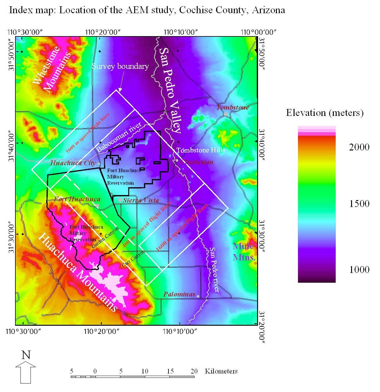
This section presents results of a qualitative and semi-quantitative interpretation of the aeromagnetic field data collected during the 1997 airborne electromagnetic survey of the Fort Huachuca Military Reservation and surrounding vicinity (Geoterrex-Dighem, 1997; see Index Map below). This survey was designed to collect time domain electromagnetic sounding and magnetic field data from above bedrock of the Huachuca Mtns., northeast across the San Pedro basin, and above bedrock of the Tombstone Hills. The main purpose of acquiring these data was to provide insight into the shallow- and intermediate-depth subsurface structure of the basin.
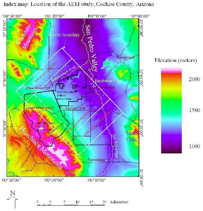
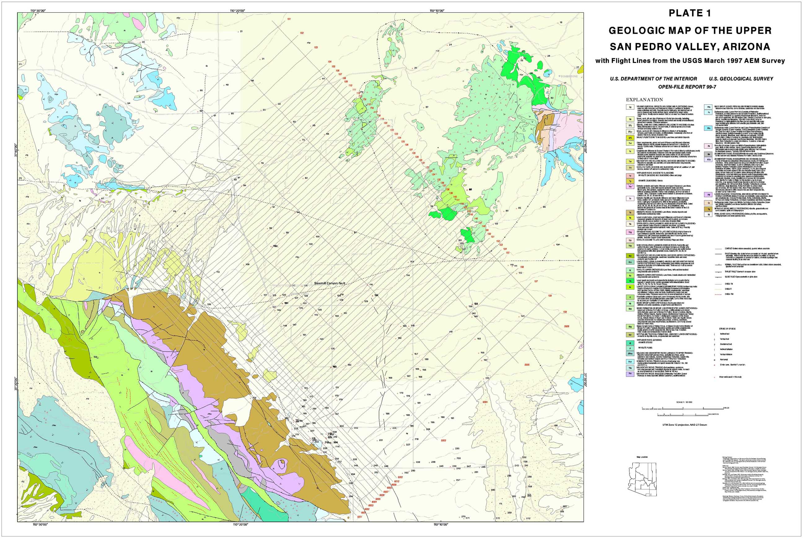
The main survey block (Index Map) consisted of lines spaced 1/4 mi. (400 m) apart along the direction N47� E with orthogonal tie lines spaced about 4 km apart. Three additional lines spaced one mi. (1.6 km) apart were appended to the northwest side of the area and four one mi. spaced lines were appended to the southeast side of the survey. The widely spaced lines were included to sample electromagnetic data over the areas of thicker basin fill as defined by models of the gravity anomaly field (Gettings and Houser, 1995). Steep relief of the Huachuca Mtns. range front necessitated flying a 4.5 km strip of the area along the southwest edge in a northwest-southeast direction, parallel to the tie lines. Location of flight lines was achieved by use of differential global positioning system equipment, post-processed for final adjusted values. The flight line paths are shown on the geologic map of the area (Pl.1), together with selected geographic information. A cesium vapor magnetometer was used to collect the data in the aircraft; this instrument has a sensitivity of 0.01 nanoTesla (nT) and a sample rate of 10 Hz. Aircraft speed was about 65m/s, so sample interval is about 6.5 m along the flight lines. The nominal magnetometer sensor height is 73m above the ground. For this survey, actual mean sensor clearance was 87m with a standard deviation of 23m and a maximum of 288m. Noise envelope for this survey was about +/- 0.5 nT. A base station magnetometer was also operated near the center of the survey area to provide data for the diurnal correction. The contractor completed corrections to the magnetic field data for diurnal drift, lag (distance behind GPS antenna), levelling (tie line intersections), and subtraction of the International Geomagnetic Reference Field computed at an altitude of 1431m above mean sea level. The contractor supplied the magnetic field data as digital files of data along the flight lines, and on a grid with an interval of 50 m. The grid file did not include the one mile spaced lines on the northwest and southeast edges of the survey area. The contractor also provided a contour map at 5nT interval created from the grid file. The magnetic field anomaly map is shown in Plate 1.1 in several renditions. The map and its digital equivalent were the primary dataset used in this interpretation. Overall, the quality of the magnetic anomaly data is very good.
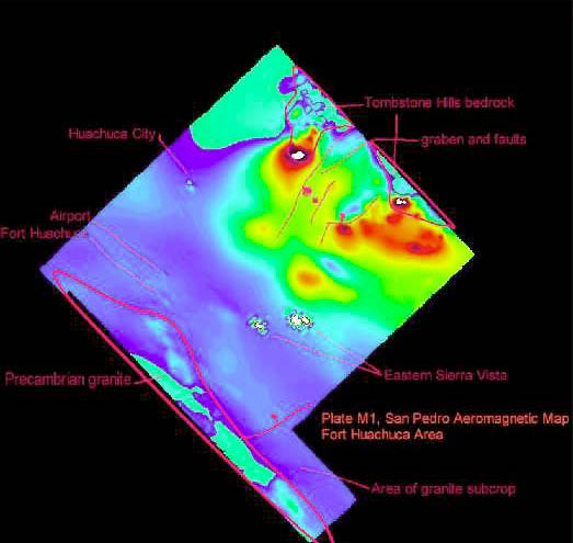
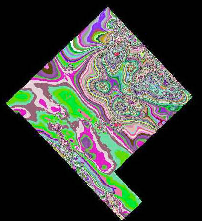
Image 2 of Plate 1.1, Random colors to show trends.
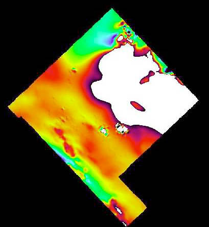
Image 3 of Plate 1.1. High intensity anomalies have been removed to emphasize low amplitude anomalies and features.
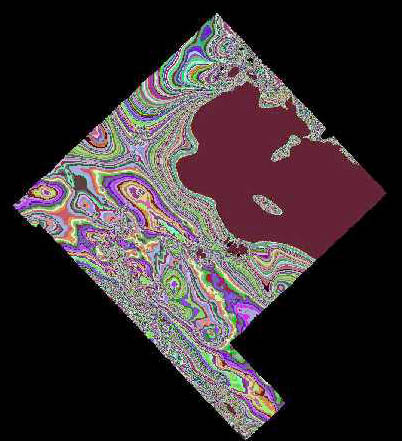
Image 4 of Plate 1.1. Random colors version of image 3 to emphasize trends.
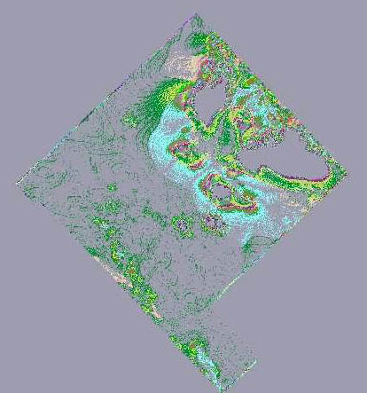
Image 5 of Plate 1.1. Magnetic anomaly field with edge enhancement operator to help delineate areas of different texture in the anomaly field.
Study of Pl. 1.1 (especially image 1) reveals that the anomaly map is composed of two main areas. The southwest half of the map is made up of smaller, more linear anomalies of amplitudes of 20-400 nT and characteristic widths of 1-3 km. These anomalies have sharper gradients near the southwest border indicating shallower depths of source, and appear to be due to sources in the Precambrian granite near the surface. This area is labeled "Precambrian granite" in image 1 of Pl. 1.1. Immediately to the northeast, the anomalies have gentler gradients over the basin fill east of bedrock, indicating larger depths to source. The northeast half of the survey area contains several large anomalies of as much as 2000 nT amplitude which are more nearly circular or equant in map view. These anomalies are about 3-5 km in diameter with moderately steep gradients indicating intermediate depth sources not obviously exposed at the surface. The extreme northeast part of the area is characterized by small areal extent anomalies of strong amplitude. These occur mainly over exposed Cretaceous volcanic rocks of the Tombstone Hills (labeled "Tombstone Hills bedrock" on image 1 of Pl. 1.1), and many of the anomalies indicate reversed magnetic polarity, particularly from line L111 to line L139 (Pl.1). Gettings and Gettings (1996) also recognized the presence of reversely polarized rocks in this area during interpretation of magnetic anomaly data collected along Charleston Road. The anomalies display several trends, defined by alignment of gradients and shapes of anomalies, which are best illustrated on images 2 and 4 of Pl. 1.1. The most dominant trend direction is approximately northwest-southeast, followed by east-west trends, and least dominant are northeast-southwest and north-south trends (however, there are several strong northeast-southwest trends in the north quarter of the survey area). Several anomalies in the southwest portion of the study area trend northwest-southeast or north-south and are cut and/or offset by east-west and northeast-southwest trends. Finally, there are several areas of high intensity, short areal dimension anomalies which correspond to structures and other man-made features in the Fort Huachuca, Sierra Vista, Sierra Vista airport, and Huachuca City areas and are labeled on image 1 of Pl. 1.1.
Aeromagnetic Data Processing
The principal objectives of the interpretation were to define depths to magnetic sources and important trends and structures that are identifiable in the magnetic anomaly field. Thus the computational effort was expended on these products rather than modeling particular anomalies to produce estimates of the shapes of the causative bodies. For both depth estimation and trend analysis, monopolar forms of the magnetic field anomaly are required. The magnetic field of the Earth in the study area has an inclination of about 60� down into the Earth, but using a mathematical transformation called "reduction to the pole" the magnetic anomaly field can be recomputed to a field with vertical magnetization inclination. The result of the reduction to the pole operation is a field which would be observed if the given field had been observed with vertical polarization, that is, as though observed at one of the Earth’s magnetic poles. If strong remnant magnetization is present in directions other than that of the Earth, the transformed field will be in error. In the study area, the remnant magnetization direction is nearly antiparallel to that of the Earth, and so does not cause serious errors. By means of Poisson’s Relation, the "pseudogravity" can also be calculated from the magnetic anomaly field. The pseudogravity field is the gravity field that would be observed if the magnetic sources were each uniformly magnetized (all in the same direction) and assuming each body has a uniform density (which may differ between bodies).
For this interpretation, the pseudogravity and reduction to the pole transformations were obtained in the frequency domain using Fast Fourier Transforms applied to the digital grid of the data. Program FFTFIL (Hildenbrand, 1983) was used to calculate the two transformations and produce a new grid for each. For both trend analysis and depth estimates, a grid of horizontal gradient magnitude was required. These were obtained using a procedure (J. Phillips, 1997) which calculates the gradients in the x- and y-directions by fitting a spline curve and then calculates the horizontal gradient magnitude value at each grid point. This finally yielded two grids of horizontal gradient, one each for the pseudogravity and reduction-to-the-pole transformation.
Depth to magnetic source was then estimated using software written by J. Phillips (1997) which calculates depth to source, an estimate of the error in depth as percent, and the azimuth of the horizontal gradient maxima, corresponding to the strike of the gradient used to estimate depth. The software calculates the depth estimates by approximating the analytic signal for horizontal gradient maxima detected by passing a window over the grid. As shown by Nabighian (1972), depth to the top of a magnetic source can be calculated from the analytic signal. Depths calculated from the horizontal gradient of the reduced-to-the-pole magnetic data estimate the depths to the top of thick magnetic sources and thus yield minimum depth values. Depths calculated from the horizontal gradient of pseudogravity correspond to depths to the top of thin magnetic sources and yield maximum depth values. Only estimates of depth with error estimates of less than plus or minus 10 percent were used. Maps of the minimum and maximum depths to source thus calculated are presented in plates 1.2 (minimum depths) and 1.3 (maximum depths). On these maps, the depth is plotted at map scale as the diameter of a circle centered at the location of the depth estimate with a straight line segment showing the azimuth of the gradient. Depths on the map are depths below the sensor and were calculated assuming a sensor terrain clearance of 120m; thus in using the maps, 120m must be subtracted from the map depth to obtain depth below the surface. As stated above, the actual mean terrain clearance for this survey was 87 m and therefore 33m should be added to get the final depth estimate; that is, the net correction is to subtract 87m. Many of the depths of interest are 500 m or less, and for these the minimum depth map value (Pl. 1.2) should be the most realistic value assuming that the magnetic sources are of the order of a km or more thick beneath the basin fill . For depths of one km or greater, the source will probably not be well approximated as thick because the igneous intrusives and volcanic rocks most likely to be the magnetic sources will be of the same order of thickness as their depth of burial. Thus for the deeper sources, a depth between the minimum (Pl. 1.2) and maximum (Pl. 1.3) will be the most likely.
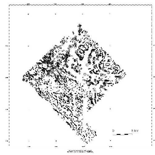
Plate 1.2. Depths to top of magnetic source estimated from reduced-to the-pole transformed magnetic anomaly data.
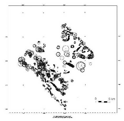
Plate 1.3. Depths to top of magnetic source computed from the pseudogravity transformed magnetic anomaly data.
Trends defined by edges of magnetic bodies were delineated by plotting the location of maxima of horizontal gradients on maps. Plotting all maxima results in a very confusing pattern from which it is difficult to draw trends, and so software was employed to select classes of maxima to plot based on their shape, continuity, and amplitude (Blakely and Simpson, 1986). This procedure was carried out for both the pseudogravity and reduced to the pole grids, with several sets of criteria. Trend lines were then compiled from these maps into a map of magnetic trends which was overlain on the original magnetic field data (Pl. 1.1) for validation. A subset of these trends was then manually extracted, choosing mainly those with continuity of a kilometer or more, to obtain a subset representing the important trends. This subset is shown on plate M4 as blue lines to distinguish them from other lines on the plate.
Interpretation
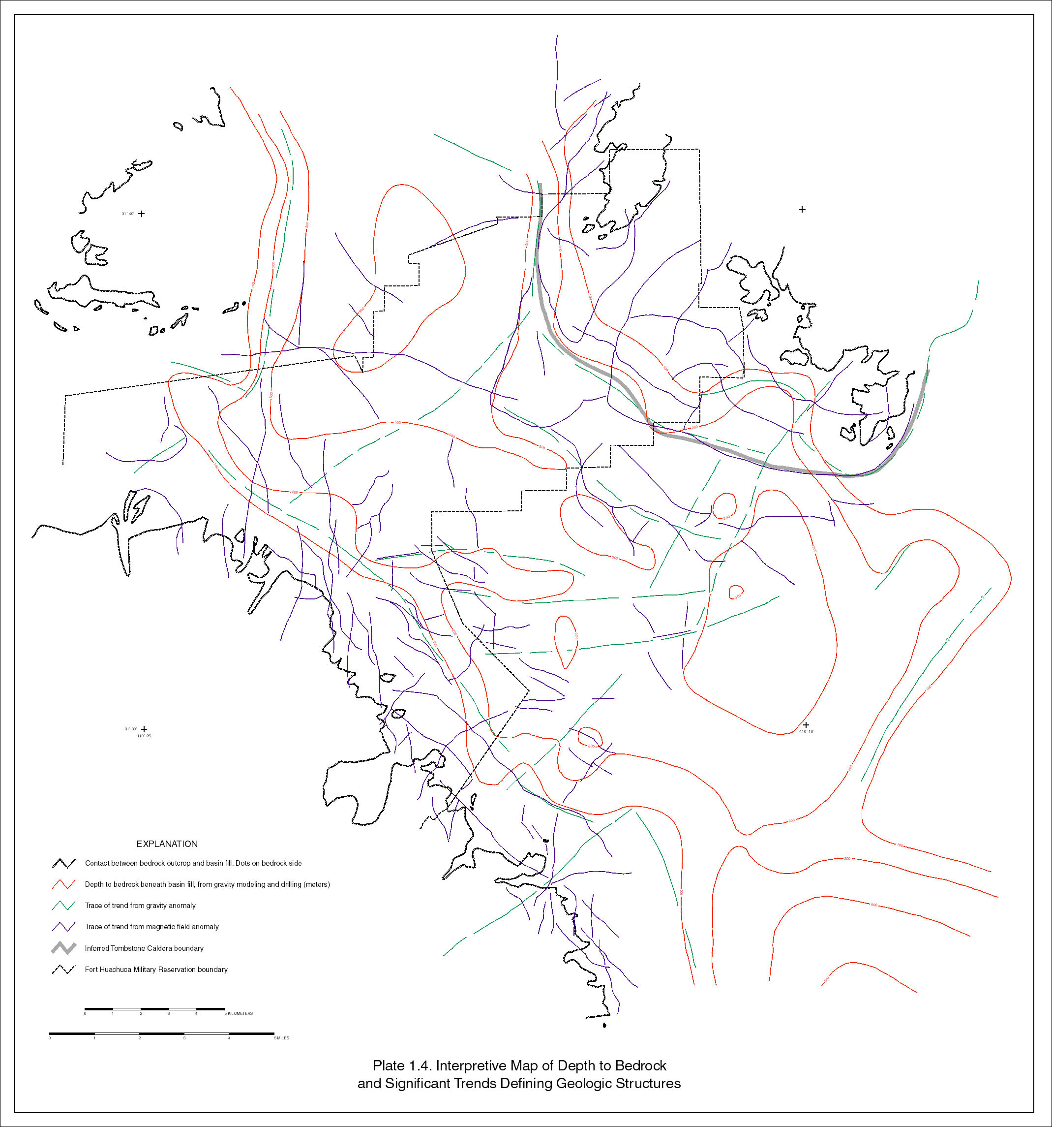
Other data and interpretive results were compiled on Pl. 1.4. These include the contact of bedrock outcrop with basin fill from Pl.1 (shown as black lines on Pl. M4) and trends from an analysis of the gravity anomaly map (Gettings and Houser, in prep), similar to that described above, shown as green lines. Also shown on Pl. 1.4 with red lines are the 100m, 200m, 500m, and 900m model depth to bedrock contours from gravity modeling constrained by drilling information (Gettings and Houser, in prep). Plates 1.1-1.4 were overlain on each other and on the geologic map (Pl.1) and topograhic map (Defense Mapping Agency, 1994) in order to study the various features and relate them to each other. Anomalies, depths and trends apparently due to surficial and manmade features were discarded from the interpretation and are not discussed here. The major results of the interpretation are discussed here, in no particular order.
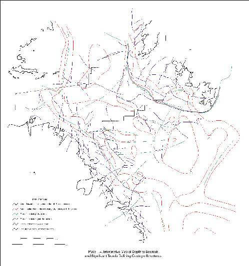
Plate 1.4. Interpretive map of depth to bedrock and significant trends defining geologic structure.
The inferred southwest margin of the Tombstone caldera (Moore, 1993) is outlined by the prominent gravity and magnetic trends and labeled "TC" on Pl. 1.4; these trends are the southwest gradient of the large intermediate-depth magnetic anomalies separating them from the two deeper anomalies to the southwest which are here interpreted to be intrusive masses lying outside the caldera at depths-to-top of 400-500 m. Depths-to top of the intermediate depth anomalies (within the caldera) are 100-300m and these anomalies are also inferred to be due to igneous intrusions, similar to the granodiorite of Granite Peak in the Whetstone Mountains (Drewes, 1980; Drewes, 1996; Gettings, 1996; Bankey and Kleinkopf, 1985) or the Schieffelin granodiorite (Moore, 1993) near Tombstone, both of which are strongly magnetic. The location of the caldera margin inferred from the geophysical data lies considerably to the west and southwest of the inferred location of Moore (1993) in the areas of cover. As shown on all the interpretive maps, northeast trending faults cut the northeastern half of the survey area, creating a graben and valley fill between the two major areas of outcrop along the northeast boundary of the area (see "graben and faults" on image 1 of Pl.1.1), and several other northeast trends which offset magnetic anomalies in areas of outcrop in the Tombstone Hills.
In general, the depth estimates from the magnetic anomaly data agree well with those from the gravity modeling if one uses the depths from the reduced-to-the-pole computation (pl.1.2). The areas of shallow bedrock ("bedrock highs") reported from drilling and gravity models (Gettings and Houser, 1995; Gettings and Houser, in prep.) are confirmed and better outlined in map view (Pl. 1.4). At the location of test well 8 (#100, Pl.1; see also Gettings and Houser, in prep.), the magnetic anomaly depth to source (Pl. 1.2) is 466m whereas the drilled depth to bedrock is 395m, so the minimum depth from the magnetic anomaly data is 74 m deeper. The drillhole geologic log describes this rock as a volcanic conglomerate, and it is here interpreted to be part of the Tombstone Caldera siliceous volcanic unit or the underlying ash flow tuff of the Bronco Volcanics (Moore, 1993) as it has a bulk density more appropriate for a tuff than for a lava (Gettings and Houser , in prep.). In either case the thickness of the tuff at this locality is unlikely to exceed approximately 150m (Moore, 1993); 61 m were penetrated in the borehole. Using the depths from the pseudogravity transform (Pl. 1.3) gives a depth 1.2 to 1.4 km for a thin source. The tuff is known to be magnetic where exposed in the Tombstone Hills; however the character of the two large magnetic anomalies on whose gradients the drillhole falls suggest a strongly magnetized thick source, probably an intrusion, rather than a thin sheet of outflow tuff from the caldera. Therefore the depth to magnetic source is here inferred to be 450-500m and due to a magnetic intrusive rock underlying the tuff penetrated by the drillhole. This intrusion is inferred to be intrusive into the rocks of the Tombstone Caldera at depth, possibly along the caldera ring fractures, but with the main mass as a sill lying outside the caldera margin.
A horst, delineated mainly by the gravity gradients, extends southwest from about 3km south of Charleston across the basin to about 2km north of the entrance to Carr Canyon is notable and contains at least two areas of depth to bedrock of 200m or less (index map and Pl.M4). Many of the magnetic anomaly trends crossed by the horst are broken or offset (Pl.M4). This horst runs beneath the sewage treatment ponds of the city of Sierra Vista and appears to have about 100m throw. The magnetic anomaly trends and depths delineate the shape of another bedrock high trending east-west beneath the city of Sierra Vista very clearly.
The northeast-southwest and east-west trends in both the gravity and magnetic anomaly data break and offset the dominant northwest-southeast trends. This pattern suggests that the whole of the survey area, which is in general a bedrock high between the subbasin at Huachuca City and the subbasin at Palominas (Gettings and Houser, 1995), is complexly faulted and fractured along principally northeast-southwest and east-west directions. Although the data are ambiguous, there is some suggestion, principally from the trends (Pl. 1.4) but also from the depths and magnetic anomaly map itself, that the northeast trends are younger and offset the east-west structures.
Immediately west of Huachuca City , and to a lesser extent to the east, there is an area of consistent depth estimates of 250-350m depth to source (Pl. 1.2) which fall in an area of 500m and 900m depth to bedrock from the gravity anomaly models (Pl. 1.4). Comparison of the anomaly responsible for these depth estimates with aeromagnetic data to the west (U.S. Geological Survey, unpublished) shows that the anomaly continues westward and shallows abruptly across a mapped fault (Pl. 1) and intensifies to well defined anomalies over areas of mapped Tertiary andesitic volcanic rocks. Therefore the area around Huachuca City is interpreted to be underlain by these volcanic (magnetic) rocks at depths of 250-350m. In outcrop to the east, it is unclear whether these rocks rest on Tertiary Pantano? Formation conglomerate or on rocks of Cretaceous age (B. Houser, personal comm., 1998). If the latter, then the subbasin defined by the part of the gravity model beneath the volcanic rocks (red contours in Pl. 1.4) would be Cretaceous in age and not a Tertiary subbasin at all. In either case, the subvolcanic rocks are probably of low permeability. Unfortunately, no wells of 250m or greater depth have been found in this area to test the volcanic rock hypothesis.
In the northwestern part of the survey area, the magnetic anomaly depth estimates provide some constraints on the magnitude of the fault offset of the bedrock of the Huachuca Mountains to the south against the Tertiary Pantano? Formation conglomerate to the north (Pl.1). The area from the fault northward to the Babocomari River has an average depth estimate of about 175m with the deepest estimates near the fault of about 300m and the shallowest nearly at the surface at the Babocomari River. Using a 10� average southward tilt obtained from the average dip of the Pantano? Formation from the geologic map (Pl.1) gives a much greater thickness (about 1600m) for the offset at the fault, so the section must be faulted in several places if it is as thin as the magnetic depth estimates suggest. Alternatively the depths could be reflecting depth to an intercalated volcanic unit as discussed above, and the total conglomerate thickness would then be greater including the conglomerate below the volcanic rocks.
Finally, the extreme south part of the study area includes granite bedrock along the southwest-most flight lines and basin fill to the northeast (Pl.1). The depth estimates (Pl. 1.2) show very shallow depth to source in the "panhandle" area of the survey, confirming that it is a shallow fill on granite bedrock pediment extending out into the basin to the northeast. To the north, the depths get deeper across the southwest trending fault where the range front fault jumps southwestward toward the Huachuca Mtns. These offsets (in map view) of the range front fault basinward to the southeast have been documented elsewhere (Gettings and Houser, 1995) but the present survey refines its location and shape. The northernmost offset is just south of the entrance to Garden Canyon (index map; the northwest boundary of the area labeled "area of granite subcrop", image 1 of Pl. 1.1), and may explain the offset in the depth to water contours in this area shown by Brown and others (1966) and other authors.
References

![]() U.S. Department of the Interior |
U.S. Geological Survey
U.S. Department of the Interior |
U.S. Geological Survey
URL: http://pubsdata.usgs.gov/pubs/of/1999/0007-b/gettings/ch1.html
Page Contact Information: GS Pubs Web Contact
Page Last Modified: Wednesday, 07-Dec-2016 17:50:58 EST
