Open-File Report 99-399
By Mark W. Bultman
Table of Contents
Part 1. Geologic Setting of the San Rafael Valley
1.1 The Regional Geology of southeastern Arizona
1.2 Geology of the San Rafael Valley
1.3 Known basin geometry and sediment fill, San Rafael basin
Part 2. Modeling the geometry of the San Rafael basin
2.3 The sediment that fills the San Rafael basin
2.4 The water table in the San Rafael basin
2.5 Density of the sedimentary fill in the San Rafael basin
2.6 Depth to bedrock in the San Rafael basin
2.7 Basin cross-sectional depth and structure modeling using a forward modeling program
3.2 Near-ground, closely spaced Earth’s total intensity magnetic field data
3.5 Estimating concealed lithology
3.6 Problems with the quantitative estimation of concealed lithology
3.7 Structural information from truck-mounted magnetometer data
Part 4. Geometry, structure, and concealed lithology of the San Rafael Basin
Figures
Figure 1. Location of the San Rafael Valley
Figure 2. West to east gravity model over the San Rafael basin
Figure 3. North to south gravity model of the San Rafael basin
Figure 4. Near-ground, closely spaced Earth’s magnetic field signal over TKg
Figure 5. Near-ground, closely spaced Earth’s magnetic field signal over JTRvs
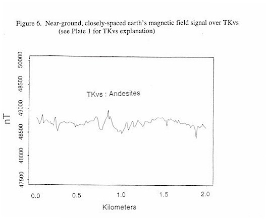
Figure 6. Near-ground, closely spaced Earth’s magnetic field signal over TKvs
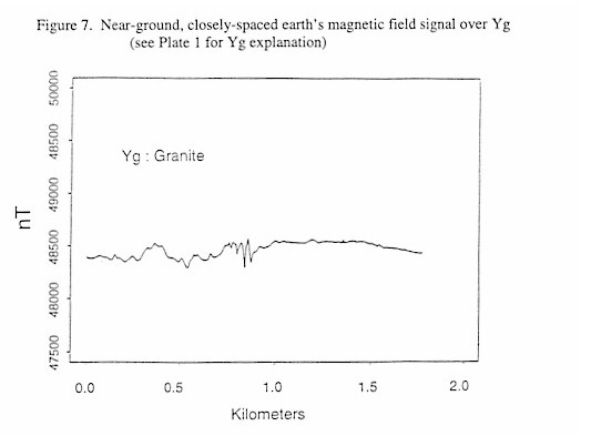
Figure 7. Near-ground, closely spaced Earth’s magnetic field signal over Yg
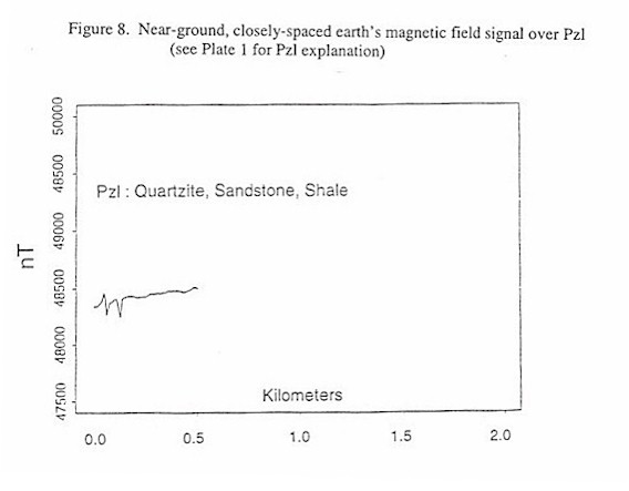
Figure 8. Near-ground, closely spaced Earth’s magnetic field signal over Pzl
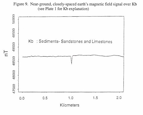
Figure 9. Near-ground, closely spaced Earth’s magnetic field signal over Kb
Figure 10. Calculating the fractal dimension for unit Kb using the rescaled Range analysis method
Figure 11. Calculation of the fractal dimension for unit Kb using the power spectrum method
Figure 12. Principal component analysis of the five textural measures for exposed lithologies
Figure 13. Example of signal form basin fill
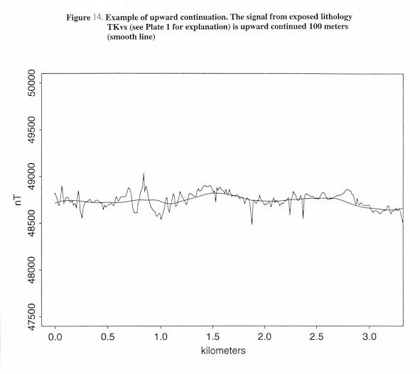
Figure 14. Example of upward continuation
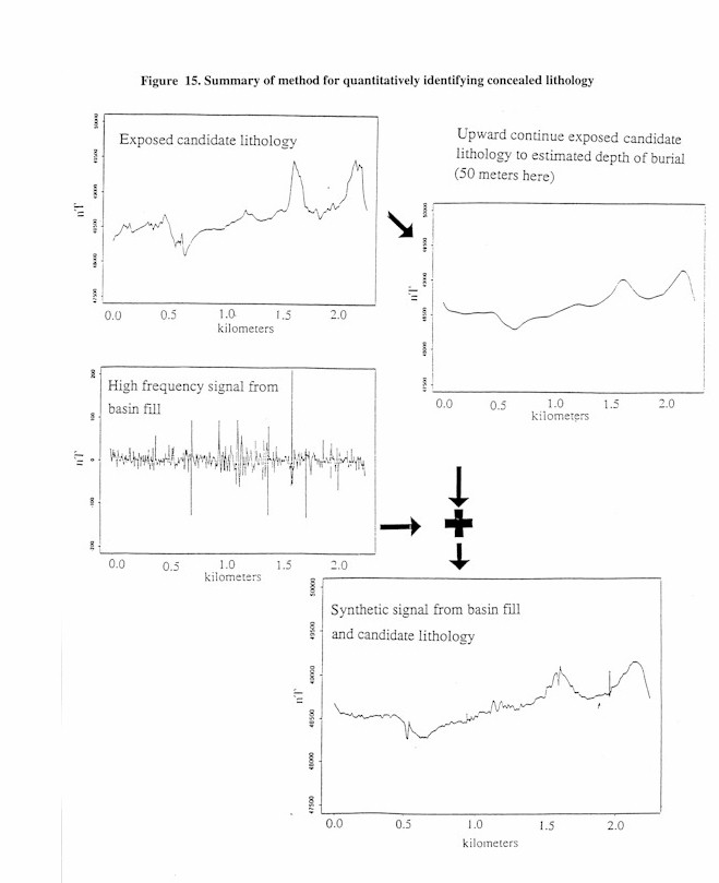
Figure 15. Summary of method for quantitatively identifying concealed lithology
Figure 16. Comparison of signal acquired over basin with synthetic signals for site 1
Figure 17. Comparison of signal acquired over basin with synthetic signals for site 2
Figure 18. Location of truck-mounted magnetometer profiles in the San Rafael Valley, Arizona
Figure 19. Earth’s magnetic field model for anomaly in profile 1
Figure 20. Modified west to east gravity model changing the density of body 6
Plates
Plate 1. Geologic map of the San Rafael Valley region
Plate 2. Complete Bouguer gravity anomaly map of the San Rafael Valley
Plate 3. Water table elevation in the San Rafael basin
Plate 4. Depth to water table in the San Rafael basin
Plate 5. The residual gravity anomaly of the San Rafael basin
Plate 6. Depth to bedrock in the San Rafael basin
Plate 7. Earth’s magnetic field anomaly map of the San Rafael Valley
Plate 8. Annotated truck-mounted magnetometer profiles in the San Rafael Valley
Plate 9. Geologic map of the San Rafael Valley region with truck-mounted magnetometer data
Plate 10. Concealed lithology of the San Rafael basin
Tables
Table 1. Deep wells in the San Rafael basin
Table 2. Water wells in the San Rafael Valley
Table 3. The density model for basin fill in the San Rafael basin
Table 4. Gravity anomaly versus depth function for the San Rafael basin
Table 5. Map units and densities of bodies used in the forward model of Figure 2
Table 6. Map units and densities of bodies used in the forward model of Figure 3
Table 7. Textural measures of Earth’s total intensity magnetic field for exposed lithologies
Table 10. Map units and densities of bodies used in the new forward model of Figure 20
The contiguous United States has been well explored for exposed conventional mineral deposits. Therefore, it is likely that many economically viable and strategically significant conventional undiscovered mineral deposits will be found in bedrock concealed beneath basin sediments. Mineral resource assessments must incorporate an understanding of the geometry, structure, and concealed lithology of basins in order to be accurate. This report presents an analysis of the basin geometry and structure of the San Rafael basin in southeastern Arizona. In addition, a new methodology for inferring concealed lithology is presented and applied in the San Rafael basin.
Gravity data is used to model the geometry of the basin using recent models of sediment density vs. depth developed in the region. This modeling indicates that the basin has a maximum depth of approximately 1.05 km plus or minus 0.10 km. In the southern portion, the basin can be modeled as an asymmetric graben faulted on the western margin. The northern portion of the basin is structurally more complex and may have high angle faults on the western, northern, and eastern margin. Near-ground closely spaced Earth’s total intensity magnetic field data is used to locate concealed faults within the basin. This data is also used to infer lithology concealed by shallow basin sediments. Airborne Earth’s total intensity magnetic field data is used to help infer concealed lithology in deep portions of the basin. The product of integrating all data and interpretations is a map which presents the geometry of the basin, faults and contacts concealed by basin sediments, and an estimate of the bedrock lithology concealed by basin sediment.
Based on basin geometry and concealed lithology, the San Rafael basin has a high potential for concealed mineral deposits on its western and northern margin. In particular, a newly discovered magnetic anomaly in the northern portion of the basin can be modeled as a granitic intrusion with highly altered margins and may represent a potential mineral resource target. Based on the permeability and porosity of upper basin fill found in nearby basins, the San Rafael basin may contain an aquifer up to 300 meters thick over a substantial area of the basin.
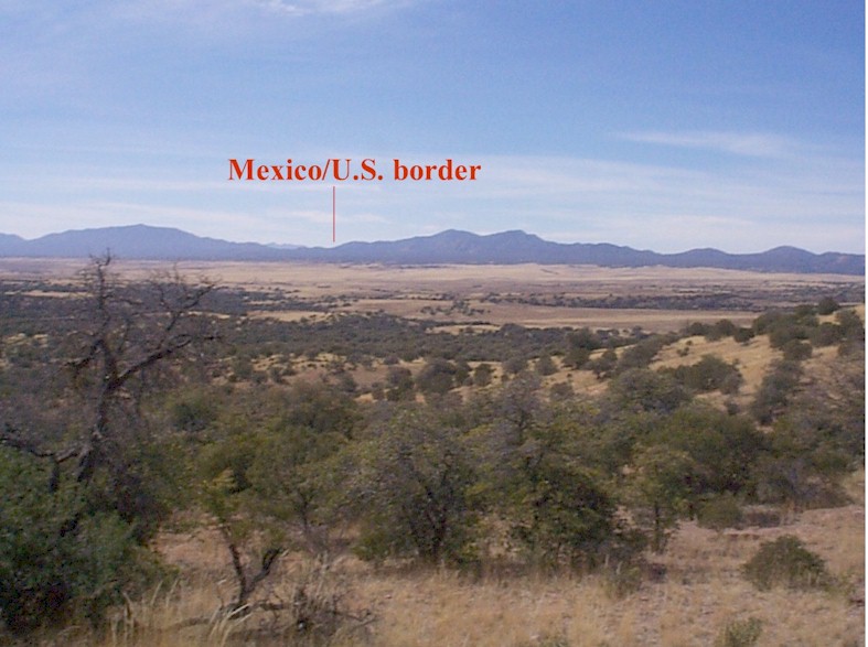
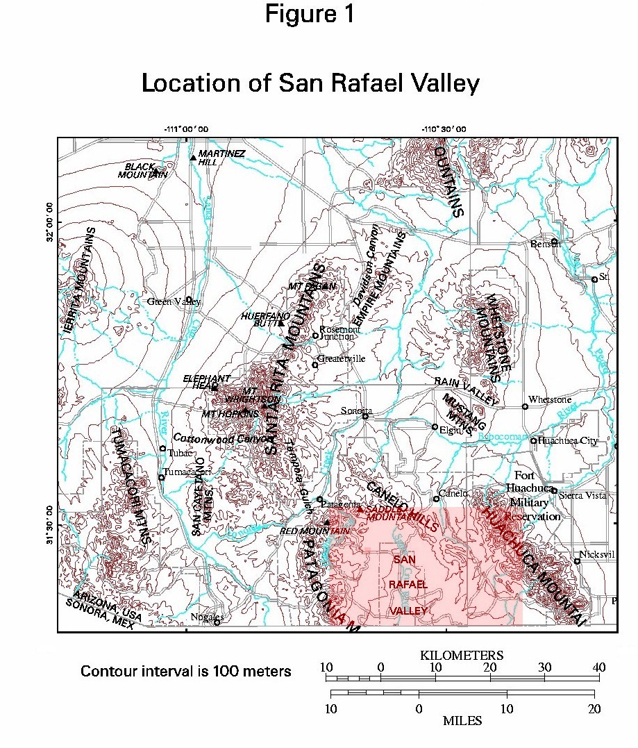
The mineral resource assessment of the Coronado National Forest was published in 1996 (Du Bray, 1996) and included work in the Patagonia Mountains, Canelo Hills, and Huachuca Mountains of southeastern Arizona. The Patagonia Mountains have a long history of mineral production and include a major porphyry copper deposit. The Huachuca mountains have produced moderate amounts of minerals including tungsten. The Canelo Hills have had little mineral production. Between these mountains lies the San Rafael Valley (Figure 1) at an elevation of about 1500 meters. The basin under the valley floor is described as a bowl shaped depression with a sediment depth of 750 to 1000 meters (Gettings, 1996). In the mineral resource assessment of the Coronado National Forest (Du Bray, 1996), parts of the San Rafael basin were determined to have a moderate probability of hosting a number of types of ore deposits. This report further addresses the geometry, structure, and concealed lithology of the San Rafael basin for the purpose of understanding its mineral resource potential. Because of the importance of water issues in southern Arizona, information on possible aquifer thickness is also provided.
Part 1 provides some background information on the geology of the southeastern Arizona and the San Rafael Valley. Part 2 uses gravity data to model the geometry and structure of the San Rafael basin. Part 3 uses near-surface closely spaced total intensity Earth’s magnetic field data to enhance the geometry and structural geology of the basin, and to make estimates of the bedrock lithology concealed below basin sediments.
The term San Rafael Valley will be used to refer to the geographic area. The term San Rafael basin will be used to refer to the tectonic depression created from basin and range faulting and the sediment that fills it. Most geologic maps that are produced in the United States are based on time-stratigraphic map units and this includes the geologic mapping used in the San Rafael Valley. Because there is no lithologic map available, this report treats map units on existing maps as if they are lithologic units. The term lithology and map unit will both be used to represent the mapped time- stratigraphic unit that, for the purposes of this report, is serving as a lithologic unit.
View of the San Rafael Valley, Arizona from the Canelo Hills (Figure 1) looking to the southwest. The U.S.- Mexico border is shown where it crosses the Patagonia Mountains.
Within this report Plates are maps that are available at a given scale, generally 1:125,000. If a Plate is too large to be displayed in this document, a smaller version of the Plate is shown. If so, a hyperlink beneath the smaller version of the Plate allows the reader to access the Plate at scale. Some small Plates are shown in their entirety in this document. PrinTable Postscript versions of all Plates are available in the postscript archive. A hyperlink to this archive can be found beneath all Plates shown in this document.
Part 1. Geologic Setting of the San Rafael Valley1.1 The regional geology of Southeastern Arizona
The San Rafael Valley is located in the southern Basin and Range physiographic province of southeastern Arizona and northern Sonora, Mexico (Figure 1). This region has seen significant deformation in the Precambrian, Mesozoic, and Cenozoic eras. The oldest exposed rocks in the region are lower Proterozoic marine sedimentary and volcanic rocks deposited at southern margin of the early N. American craton (Silver, 1978). These rocks were metamorphosed in the early Proterozoic to form the Pinal schist. The Pinal schist was intruded by granitic rocks during 2 subsequent periods, 1.65 and 1.45 Ga (Peterson, 1988). The intrusive phase was followed by uplift and 200 to 300 million years of erosion to a low relief landscape. Around 1.2 Ga, Apache group sedimentary rocks were deposited in the region that is now southeastern Arizona, but none have been mapped in the San Rafael basin area.
Following the deposition of the Apache Group rocks, there is no geologic record for the following 500 million years (Peterson, 1988). The Paleozoic rocks in the region were deposited in the Cambrian and Late Devonian through the Permian (Pierce, 1976). They represent many transgressive-regressive sequences and form hundreds to thousands of meters of limestones, shales, and sandstones (Peterson, 1988). The lower portion of the Paleozoic sequence is the most common host to ore deposits in the region (Drewes, 1996).
During the Mesozoic, the region that is now southeastern Arizona underwent an orogenic event with extensive magmatism, deformation, and metamorphism. There is evidence of vertical movement from the Triassic to mid-Cretaceous along northwest trending fault zones in the region. The Early- and Middle-Jurassic is marked by extensive rhyolitic to dacitic volcanism and numerous granite, monzonite, and quartz monzonite intrusives.
In the late Jurassic and Cretaceous there was a marked decrease in magmatism and the region experienced block faulting and extensive deposition of thousands of meters of non-marine clastic rocks that now form the Bisbee Group. (after Peterson, 1988; Drewes and Finnell, 1968; Drewes, 1996).
The Late Cretaceous and Early Tertiary was a period of active tectonism generally referred to as the Laramide Orogeny. This period was characterized by northeast- southwest regional compression and low angle thrusting. Between 75 and 65 Ma extensive volcanism formed large andesitic stratavolcanoes and collapse calderas resulting from the eruption of rhyolitic ash (Peterson, 1988). This volcanism was contemporaneous with the emplacement of intermediate composition intrusives (Titley, 1982).
The Laramide was followed by a period of quiescence and erosion in the Eocene. and then renewed tectonism in the Oligocene. Massive late Oligocene-early Miocene calc- alkaline volcanism and plutonism and associated sedimentation followed. Crustal extension during this time period formed gently dipping normal-displacement shear zones of regional extent that penetrated into the middle of the crust (Peterson, 1988). Late Miocence to Pliocene episodes of basin and range block faulting placed up to 3 km of non-marine clastic sediments and evaporites in the basins. Basin filling was followed in some areas by stream downcutting, the development of terraces, and valley unloading (Scarborough and Pierce, 1978).
1.2 The geology of the San Rafael Valley
The physiography of southeastern Arizona has been described as a terrain of alternating fault bounded linear mountain ranges and sediment filled basin. It began to form about 17Ma in southeastern Arizona as the result of dominantly northeast/west- southwest directed crustal extension. (Gettings and Houser, 1999) The basins are the result of several episodes of extension which leads to shapes that can be quite complex. The San Rafael Valley is surrounded by the Patagonia Mountains to the west, the Canelo Hills to the north and east, and the Huachuca Mountains to the east.
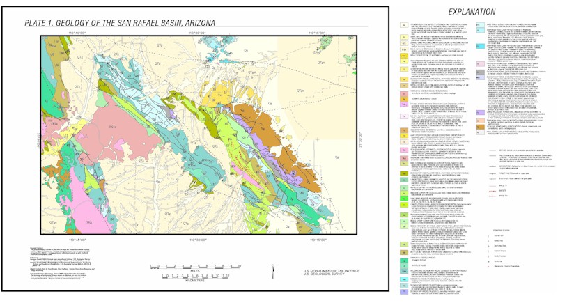
The geology of the San Rafael Valley region is shown on Plate 1. The geologic data displayed on this map are based primarily on Drewes (1996). Some modifications have been made in the basin sediments by B. B. Houser of the U.S. Geological Survey, Tucson Arizona. The map was digitized at the U.S.G.S. Geologic Division Southwest Field Office (Kneale et al, 1997) and exists as a digital database.
Click here to display Plate 1 at scale (large JPEG file)
Click here to go to the Postscript archive for Plate 1
The Patagonia Mountains are a generally a granitic terrane that includes some Proterozoic granite and a large stack of Jurrasic and Late Cretaceous age granite. Smaller regions within this terrane contain Paleozic and Mesozoic sedimentary rocks. Cretaceous or early Tertiary volcanic rocks are common to the northeast, just north of the San Rafael basin. The Patagonia mountains are noted for their abundant mineralization which includes copper, lead, zinc, molybdenum, manganese, silver, and gold metalization occurs in vein, skarn, polymetallic replacement, and porphyry copper deposits (Drewes, 1996).
The Canelo Hills are comprised of volcanic and sedimentary rock cut by a few small intrusive bodies and many steep faults (Drewes, 1996). Mineralization in this area is sparse. The Huachuca Mountains are comprised of Paleozoic and Mesozoic rocks. These rocks overlie a Proterozoic granitic basement cut by large Jurassic and small late Cretaceous granitic bodies (Drewes, 1996). The region is moderately mineralized and includes base and precious metals in polymetallic replacement deposits along northeast to east striking faults. Tungsten is present in northwest striking quartz veins and some gold has been produced from placer deposits. The Canelo Hills and the Huachuca Mountains are both cut by northwest striking steep faults that are splays of the Sawmill Canyon-Kino Springs fault system (Drewes, 1996).
1.3 Known basin geometry and fill, San Rafael basin
The San Rafael basin has been analyzed based on its gravity anomaly using a simple model of vertical cylinders (Gettings, 1996). The results of this modeling indicate the basin is a bowl shaped depression that is 750 to 1000 meters deep based on a density contrast of 0.4 to 0.3 g/cc. Gettings (1996, p.96), also indicates that portion of the basin in the Coronado National Forest is only 300 to 500 meters deep.
At least two ages of basin fill can be detected in most basins of southeast Arizona (Gettings and Houser, 1997). The older basin fill can be moderately deformed and is generally more consolidated and denser due to diagenetic processes that alter the mineralogy of the of the matrix of the sediment and fill the pore spaces. The younger basin fill is generally poorly consolidated to unconsolidated. In the San Rafael basin, the older fill is exposed only in the very northwest corner of the basin and is generally dipping 10 to 20 degrees to the south or south east (B.B. Houser, oral comm., 1997). This older basin fill is not yet mapped in this area The density contrast between these two units is sufficient that it needs to be accounted for when modeling the basin geometry. The upper basin fill unit is, in general, the only good aquifer in most basins in southeastern Arizona.
Part 2. Modeling the geometry of the San Rafael basin2.1 Introduction
The geometry of the San Rafael basin was modeled principally from gravity data. Several recent studies of nearby basins (Gettings and Gettings, 1995; Gettings and Houser, 1997; Gettings and Houser, 1999) have detailed an accurate density-depth model for basin sediments in the region. This makes using a gravity based three-dimensional model appropriate and probably more accurate than two-dimension gravity and magnetic modeling. Aeromagnetic and ground based magnetic data will be used later in this report to enhance the gravity model of basin geometry and add structural and lithologic information.
The geometry was modeled by estimating a density depth function for the basin and then using this function to estimate the gravity anomaly due to a stack of vertical cylinders of varying radii. From the gravity anomaly data, a gravity anomaly vs. depth function will then be built. The gravity anomaly vs. depth function will be used in a least squares procedure to calculate the depth to bedrock over the entire basin.
Gravity profile data was used to model the basin geometry and structure and to verify the calculation of depth to bedrock described above. Two profiles, one west to east and the other north to south, will be used to try to produce an accurate cross section of the basin sediments and bedrock in the San Rafael basin.
2.2 Gravity data compilation
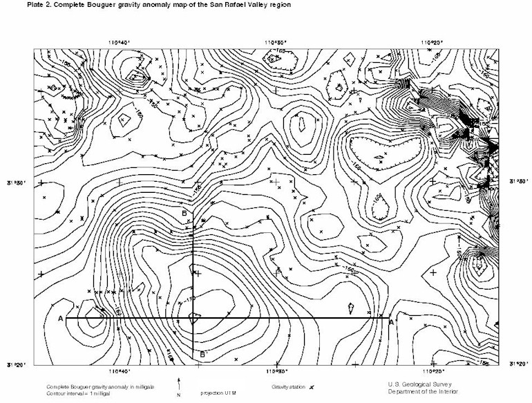
A complete Bouguer gravity anomaly database was built for the Coronado National Forest mineral resource assessment (Du Bray, 1996; Gettings, 1996) and will be utilized for this study. This includes eleven stations acquired and reduced by the author in the eastern San Rafael valley. For a gravity study on a basin the size of the San Rafael, it would be ideal to have enough gravity stations to produce a gravity anomaly grid with a cell size of 0.5 km or smaller. This shortage of gravity stations occurs mostly in the Huachua Mountains, the Canelo Hills, and the Patagonia Mountains, but many parts of the San Rafael basin could also use more gravity stations. Given the lack of gravity station coverage, a gridding interval of 1 kilometer was chosen and the data were gridded with a minimum curvature routine. This grid was contoured to produce the complete Bouguer gravity anomaly map which is displayed in Plate 2. Each gravity station (that is used in the compilation of this map) is displayed as an "X" in Plate 2.
Click here to display Plate 2 at scale
Click here to go to the Postscript archive for Plate 2
2.3 The sediment that fills the San Rafael basin
The sediments that fill Cenozoic basins in the Basin and Range Province of southern Arizona are usually defined as the detritus that accumulates in structural basins that had more or less modern configurations (Gettings and Houser, 1997). At least two ages of basin fill can be distinguished in most basins in southeastern Arizona (Houser, 1985). This is the case in the Santa Cruz basin which lies to the west of the San Rafael basin. The basin stratigraphy here can be seperated into two units based on age and consolidation. The lower basin fill unit is probably lower- and middle-Miocene in age and is poorly to moderately well consolidated. In the Santa Cruz basin this unit is the Nogales Formation. The upper basin fill unit is upper-Miocene to lower-Pleistocene and is unconsolidated to poorly consolidated. These basin fill units are overlain by Holocene surficial deposits including alluvium of stream channels, flood plains, and terraces which are unconsolidated overall but locally well indurated (Gettings and Houser, 1997). The upper basin fill unit and the thin Holocene surficial deposits are combined into one unit for the purpose of gravity modeling, this unit is called the upper basin fill unit.
Recent work on the San Pedro basin, to the east of the San Rafael basin, indicates that older mid-Tertiary conglomerate units such as the Pantano Formation may also constitute a large percentage of the basin fill (Gettings and Houser, 1999). In the San Pedro basin two basin fill units are also recognized. The Pantano Formation makes up the lower consolidated basin fill while younger poorly consolidated alluvium makes up the upper basin fill.
Information from deep wells in the San Rafael basin indicates that there are also at least two recognizable units of basin fill. While this information is limited, because there are only 3 wells deep enough to penetrate the lower basin fill unit, it indicates that the stratigraphy of the basin fill in the San Rafael basin may resemble that to the basins adjacent to it. Houser (oral communication, 1999) has indicated that the lower basin fill in the San Rafael basin, which outcrops only in the far northwest portion of the basin, is likely analogous to Nogales Formation to the west. Therefore, two units of basin fill will be used to model the stratigraphy of the San Rafael basin for the purpose of gravity modeling. The lower basin fill unit is the Nogales formation (probably lower and middle Miocene and poorly to moderately well consolidated), the upper basin fill unit is composed of younger (upper Miocene to lower Pleistocene) unconsolidated to poorly consolidated alluvium.
The three deep wells in the basin were mineral exploration wells that were drilled in the 1970’s. While no well reached bedrock, they all penetrated the lower basin fill and give some indication of the thickness of upper basin fill. Information on these wells, and their drilling logs, is given in Table 1.
Table 1. Deep wells in the San Rafael basin
| Location | Date | Total Depth (ft) | Depth to water (ft) | Drillers log | |
|---|---|---|---|---|---|
| 1. T-23S R-17E Sec-14 | 1970 | 981 | 12 | 0-5 feet: | top soil |
| 5-100 feet: | boulders | ||||
| 100-225 feet: | conglomerate | ||||
| 225-750 feet: | hard conglomerate | ||||
| 750-950 feet: | hard conglomerate | ||||
| 950-981 feet: | extra hard conglomerate | ||||
| 2. T-23S R-17E Sec-17 | 1977 | 1893 | 344 | 0-350 feet: | Unconsolidated silt and gravel |
| 350-1892 feet: | Consolidated sand and gravel | ||||
| 3. T-23S R-17E Sec-9 | 1977 | 1996 | 215 | 0-900 feet: | Unconsolidated silt and gravel |
| 900-1996 feet: | Consolidated sand and gravel |
Based on Table 1, the depth to Nogales formation is determined to be 950 feet deep at well 1, 350 feet deep at well 2, and 900 feet deep at well number 3. Given that the Nogales outcrops in only a small portion of the basin, and based on the locations and depths of the information from Table 1, it appears that the upper basin fill is thinnest on the west side of the basin and thickens to the east and to the south. The 900 foot thickness of upper basin fill from well three will be used to approximate its average thickness over the basin. The lower basin fill unit completes the rest of the basin fill from under the upper basin fill to the bedrock.
2.4 The water table in the San Rafael basin
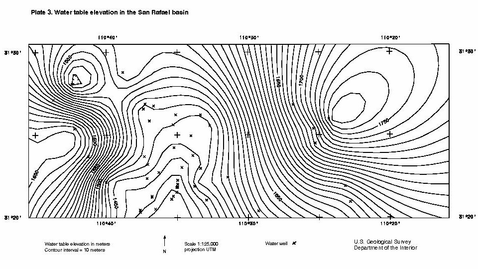
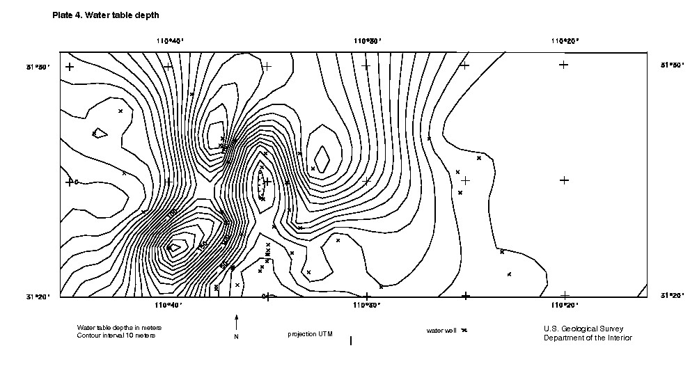
Table 2 is a complete listing of all recorded water wells in the San Rafael Valley. It was downloaded in September of 1998 from the Arizona Ground Water Site Inventory Database which is maintained by the Arizona Department of Water Resources. This database includes information of the location, well collar elevation, and water elevation of forty water wells in the San Rafael basin. The data from Table 2 are plotted in Plate 3 (water table elevation) and Plate 4 (depth to water). The data from Table 2 and the contour maps of Plates 3 and 4 indicate that the location of the water table is quite variable in the San Rafael basin, but that in the center of the basin there is a large area where it is remains near the surface. This area lies along the path of the Santa Cruz river which begins in the northern San Rafael Valley.
Table 2. Water wells in the San Rafael Valley
| ID number | Township- Range | Long. | Lat. | Depth | Well collar |
| (+110 W) | (+31 N) | to water (ft) | elevation (ft) | ||
| 311959110372001 | D-24-17 21BDD | .622 | .333 | 26.7 [1987 ] |
4692 |
| 312020110373701 | D-24-17 21BBB | .627 | .339 | 27.5 [1987 ] |
4730 |
| 312024110291901 | D-24-18 14CDC | .488 | .340 | 30.2 [1987 ] |
5010 |
| 312026110373801 | D-24-17 16CCC | .627 | .341 | 21 [1987 ] |
4725 |
| 312031110363201 | D-24-17 15CCA | .609 | .342 | 16.3 [1987 ] |
4680 |
| 312057110224701 | D-24-19 14ABA | .380 | .349 | 13.9 [1987 ] |
5250 |
| 312103110325601 | D-24-18 18ABD | .549 | .351 | 38.2 [1987 ] |
4777 |
| 312109110352501 | D-24-17 14BAB | .590 | .352 | 7.8 [1996 ] |
4645 |
| 312116110351701 | D-24-17 11DCB | .588 | .355 | 8.38 [1987 ] |
4648 |
| 312117110364701 | D-24-17 9DDD1 | .613 | .354 | 15 [1982 ] |
4725 |
| 312118110364701 | D-24-17 9DDD2 | .613 | .355 | 10.3 [1987 ] |
4722 |
| 312119110351701 | D-24-17 11CDA | .588 | .355 | 5.01 [1983 ] |
4650 |
| 312128110350201 | D-24-17 11DBA | .584 | .359 | 7.4 [1987 ] |
4662 |
| 312152110345901 | D-24-17 11ABD2 | .583 | .364 | 9.52 [1987 ] |
4676 |
| 312152110350201 | D-24-17 11ABD1 | .584 | .364 | 10.16 [1987 ] |
4676 |
| 312153110231101 | D-24-19 11BAB | .386 | .365 | 9.2 [1987 ] |
5310 |
| 312153110334801 | D-24-17 12AAC | .563 | .365 | 10 [1987 ] |
4802 |
| 312203110345801 | D-24-17 11ABA | .583 | .367 | 13.02 [1987 ] |
4680 |
| 312207110400301 | D-24-16 12BAB | .667 | .369 | 198.6 [1996 ] |
4998 |
| 312221110352301 | D-24-17 02DCA | .583 | .371 | 16.14 [1987 ] |
4690 |
| 312223110371001 | D-24-17 04DBC | .619 | .373 | 99.52 [1987 ] |
4842 |
| 312227110312601 | D-24-18 04CBA | .524 | .374 | 16.31 [1987 ] |
4902 |
| 312247110362401 | D-24-17 03BDB | .605 | .379 | 42.05 [1987 ] |
4775 |
| 312258110332001 | D-24-18 06BAB | .556 | .383 | 78.2 [1987 ] |
4830 |
| 312302110344101 | D-23-17 36CCC | .578 | .384 | 30.8 [1987 ] |
4726 |
| 312314110370501 | D-23-17 33DBC | .618 | .387 | 135.2 [1996 ] |
4928 |
| 312342110411701 | D-23-16 35BB | .688 | .395 | 10.7 [1987 ] |
5300 |
| 312343110371901 | D-23-17 33BAA | .622 | .395 | 110 [1987 ] |
4920 |
| 312345110335401 | D-23-17 36AAB | .565 | .396 | 47.3 [1987 ] |
4805 |
| 312417110351401 | D-23-17 26BDD | .587 | .404 | 7.1 [1996 ] |
4755 |
| 312428110251701 | D-23-19 28BBD1 | .421 | .408 | 15.2 [1987 ] |
5580 |
| 312457110340101 | D-23-17 24DBD | .567 | .416 | 49.8 [1987 ] |
4824 |
| 312523110252201 | D-23-19 28BCB | .423 | .423 | 17.4 [1987 ] |
5575 |
| 312526110421601 | D-23-16 22B | .704 | .423 | 9.1 [1987 ] |
5410 |
| 312534110324201 | D-23-18 18DDD | .545 | .426 | 150.3 [1987 ] |
4926 |
| 312538110351601 | D-23-17 14CDD | .588 | .427 | 8.15 [1987 ] |
4801 |
| 312552110365601 | D-23-17 16DAC | .616 | .431 | 119.5 [1996 ] |
4915 |
| 312600110241701 | D-23-19 15BCA | .405 | .433 | 12.8 [1987 ] |
5819 |
| 312613110350601 | D-23-17 14ABC | .585 | .437 | 15.6 [1987 ] |
4815 |
| 312614110332101 | D-23-18 18BAC | .556 | .437 | 121.5 [1987 ] |
4912 |
| 312636110372601 | D-23-17 09CDB | .623 | .443 | 184.3 [1987 ] |
4975 |
| 312647110364101 | D-23-17 10CBC2 | .611 | .446 | 108.1 [1987 ] |
4946 |
| 312649110265001 | D-23-19 07ACD | .447 | .447 | 16.6 [1987 ] |
5530 |
| 312652110371401 | D-23-17 09CAA2 | .621 | .448 | 175.3 [1982 ] |
5005 |
| 312707110434301 | D-23-16 08ABD | .729 | .452 | 22 [1987 ] |
5175 |
| 312803110422601 | D-23-16 03BB | .707 | .468 | 9 [1987 ] |
4822 |
| 312848110384801 | D-22-17 31ADA | .647 | .480 | 115.2 [1996 ] |
5145 |
Click here to go to the Postscript archive for Plate 3
Click here to go to the Postscript archive for Plate 4
2.5 Density of the sedimentary fill in the San Rafael basin
Gettings and Houser (1999) report the saturated bulk density of Nogales formation to be 2.32 g/cc and that Figure will be used in this study. It is worth noting that the Pantano Formation, which represents the consolidated lower basin fill unit in the San Pedro basin has a very similar density of 2.35 g/cc.
The density of the upper basin fill is more complex. This unit may or may not be saturated and has a tendency to compress and become more dense with depth. Gettings and Houser (1999) used geophysical logs of a petroleum exploration well to model densities in the upper basin fill in the San Pedro basin to the east. While the density derived from this log can be modeled with a smooth function, density functions that change with depth present analytical difficulties in gravity modeling. So the density function is compartmentalized into several layers. The upper basin fill in the San Rafael will use the same density depth function used by Getting and Houser (1999). The depths have been changed slighly for simplicity, to try to reflect the water table in the San Rafael basin, and because the depth to the consolidated lower basin fill is thought to be deeper in the San Rafael. Based on Plate 4, a water table depth of 10 meters was chosen to accurately reflect the value in the center of the basin. The density depth model for the San Rafel basin is shown in Table 3.
Table 3. The density model for basin fill in the San Rafael basin
| Unit | depth interval | density | density contrast |
| (meters) | (g/cc) | (based on 2.65 g/cc bedrock) | |
| Upper basin fill-dry | 0 to10 | 1.85 | -0.800 |
| Upper basin fill-dry/saturated | 10 to 100 | 2.10 | -0.550 |
| Upper basin fill-saturated | 100 to 150 | 2.20 | -0.450 |
| Upper basin fill-saturated | 150 to 275 | 2.27 | -0.380 |
| Nogales Formation | 275 to bedrock | 2.32 | -0.330 |
The average density (weighted by interval thickness) for the upper basin fill is 2.19. Gettings and Houser calculate the density of saturated upper basin fill in the Santa Cruz basin to be 2.24 g/cc, so 2.19 is thought to provide a fairly good representation of upper basin fill which contains some unsaturated and partly saturated sediments, but is mostly composed of saturated sediments. For simplicity, when the upper fill layer is treated as a whole (for two-dimensional profile modeling) it is assigned a density 2.20 g/cc.
2.6 Depth to bedrock in the San Rafael basin
Two methods will be used to model basin depth. The first is based on Gettings and Houser (1999). This method uses the complete Bouguer gravity anomaly due to the sediment fill of the basin alone to produce a map of depth to bedrock. The second method will use complete Bouguer gravity anomaly profiles to model cross sections of the San Rafael basin using a forward modeling tool.
The gravity anomaly due to the sediment fill of a basin can be used to build a model of the geometry of the basin fill-bedrock contact. In order to obtain this anomaly, it is necessary to separate the observed anomaly, which is due to the gravity anomaly from all sources, from the anomaly due only to basin fill. Gettings and Houser (1999), used a method modified from Saltus and Jachens (1995). This method is based on the assumption that the rocks exposed in the adjacent ranges are likely to be the same as the rocks that underlie the basin. The regional field is then built by using gravity stations that lie only on bedrock and generating a coarse interval grid (large cell size) from these stations which produces a smoothed gravity anomaly map. This regional gravity anomaly map was then subtracted from the complete Bouguer gravity anomaly grid in order to obtain a residual gravity anomaly grid due only to the sediments fill of the basin.
For three reasons, the separation of the gravity anomaly due to basin fill in the San Rafael basin was done differently. First, there are few gravity stations on the ranges adjacent to the basin meaning that a regional gravity anomaly map in this area would be based on very few data points. Second, the geology of the adjacent ranges is complex, and the gravity stations are clustered in only a few places, it is likely that a regional field obtained only from these stations could be biased based on the lithology where the stations occur. Third, no appropriate gravity map could be built in either the basin or the ranges to the south of the U.S. border in the San Rafael Valley region.
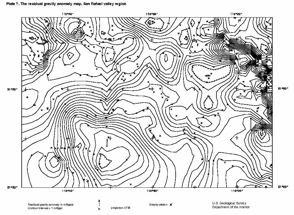
Since the study area is small and the basin fairly symmetrical, the regional field can be approximated by observing the value of the complete Bouguer gravity anomaly contours that overlap onto bedrock at the basin margin. The negative gravity anomaly due to the basin will carry slightly onto the bedrock exposed in the ranges and the first contour of a map contoured at 1 milligal interval should be a good representation of the regional field. On the eastern margin of the basin the –160 milligal contour was used. On the western margin and northwestern margin the -158 milligal contour was used. The northern margin of the basin is complicated structurally and contains shallow basin fill making it hard to find the appropriate anomaly. In addition, there is no bedrock exposed in the southern portion of the study area. For these reasons, the regional field was adjusted to represent an easterly dipping plane with a value of -158 milligals just to the west of the basin and –160 milligals just to the east of the basin. The plane has no north-south component of dip. This regional grid was subtracted from the complete Bouguer gravity anomaly grid to yield the residual gravity anomaly grid due to basin sediments. This map was contoured and is displayed in Plate 5.
Click here to go to the Postscript archive for Plate 5
Modeling software that allows the user to specify a vertical stack of cylinders with varying radii and density was used to develop a gravity anomaly versus depth function. The basin depth-density function from Table 3 was used as input. In the center of the basin a cylinder model that represents the entire basin was used and is referred to as the basin model. Cylinders near the surface had a radius of 6 kilometers and the radius gradually decreased with depth. Near the edge of the basin, a model with all cylinders having a radius of 1 kilometers at the surface and less than a kilometer at depth was used to generate values. This is the referred to as the narrow model. To represent regions intermediate between the basin and the narrow model, an intermediate model with cylinder of radius 2 kilometers at the surface narrowing to less than a kilometer at depth was used. This is referred to as the intermediate model. While several other techniques were used to model the depth of the basin near its margin, the narrow and intermediate models were as good or better than any based on the limited knowledge of the basin depth available (primarily the 3 deep exploration wells). The output from this modeling software is an estimated depth to bedrock for each gravity anomaly value for a given depth-density model (basin, intermediate, or narrow). These were used to build the gravity anomaly versus depth function.
For residual gravity anomalies from –1 to –5 milligals the narrow model was used to generate the anomaly versus depth function. This range of anomalies occurs near the margin of the basin and the narrow model will most accurately reflect the shape of this mostly fault bounded basin. For residual gravity anomalies from –6 to –9 milligals, the intermediate model was used. For the gravity anomaly values -6 and –9 milligals, linear interpolation was used to integrate this model into the narrow and basin models. Residual gravity anomaly values of –10 through –13 milligals used the basin model to generate the gravity anomaly versus depth function. The final gravity anomaly versus depth model used in the San Rafael basin is displayed in Table 4.
Table 4. Gravity anomaly versus depth function used in the San Rafael basin
| Gravity Anomaly | Basin depth |
|---|---|
| (mgals) | (km) |
| -1.0 | 0.040 |
| -2.0 | 0.090 |
| -3.0 | 0.143 |
| -4.0 | 0.218 |
| -5.0 | 0.302 |
| -6.0 | 0.384 |
| -7.0 | 0.447 |
| -8.0 | 0.542 |
| -9.0 | 0.611 |
| -10.0 | 0.665 |
| -11.0 | 0.755 |
| -12.0 | 0.901 |
| -13.0 | 1.025 |
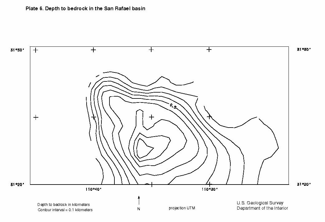
The gravity anomaly versus basin depth model is input into a program that uses a quadratic interpolation to interpret the basin depth from the residual gravity anomaly grid. The resulting depth to bedrock map is displayed in Plate 6. Using this technique, the basin models to have a maximum depth of slightly less than 1 kilometer. Plate 6 displays what appears to be fault bounded margins on the west, north, and northeast side of the basin due to the continuous extend of steep gradients of depth.
Click here to go to the Postscript archive for Plate 6
2.7 Basin cross- sectional depth and structure modeling using a forward modeling program
To verify and complement the basin depth modeling above, additional modeling was done using a 2-D forward modeling program called SAKI (Webring, 1985). The modeling procedure was initiated with a reasonable geologic cross section and reasonable densities based on the geology observed at the basin margin. The structure and physical properties are then adjusted until the modeled values (based on forward modeling) match the observed values.
Figure 2 displays the results of a west to east gravity profile and geologic cross section across the basin (A-A’ in Plate 2). The location of this profile was chosen so that it: 1) intersects the central basin gravity low; 2) is close to a west to east traverse of gravity stations down the eastern side of the Patagonia Mountains and into the basin; and 3) has some gravity stations controlling contours in the eastern portion of the basin.
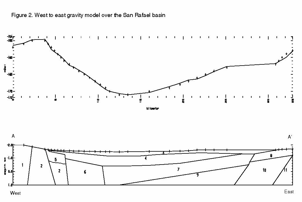
The west side of this profile begins in the granite that cores the Patagonia Mountains (TKg-body 1 in Figure 2), moves into Paleozoic sediments (PPn-body 2) that likely contain limestone or dolomite since they require a high density to model properly. Next, the profile enters Triasic-Jurrassic volcanic sediments (JTRvs-body 5) and then goes into basin sediments. The profile exits the basin on the west in Cretacoues andesites (Ka-body 8).
The basin models best with a series of step down faults on the western margin that offset bodies 2, 5, and 6. Body 6 models best as a high density unit, probably a Paleozoic one with more limestone than body 2. The lowest portion of the basin, between body 6 and body 7 is likely a fault. The eastern margin of the basin has a more gentle gravity gradient and can be modeled as dipping Bisbee Formation (body 7). The thickness modeled here (about a kilometer) is acceptable for the Bisbee formation in this region. Body 8 is Cretaceous andesite (Ka) and many andesites in this area have densities in the 2.5 g/cc region (Gettings, oral communication, 1998). The fault between bodies 7 and 8 is extrapolated from a fault observed in the mapped geology (Plate 1) and works in this model.
The basin was modeled with a density of 2.20 g/cc for the upper basin fill and 2.32 g/cc for the lower basin fill (Nogales Formation, body 4). The upper basin fill starts out thin (~100 meters) at the western edge of the basin. This coincides with the thickness of upper basin fill in deep well number 2 to the north of this profile (Table 3). The upper basin fill thickens to about 300 meters in the central and eastern portion of the basin. The basin models indicate a maximum depth of 1.05 kilometers for the combined upper and lower basin fill. Figure 2 indicates that the San Rafael basin, at least in the southern portion, can be modeled as a half-graben faulted on the western margin.
It should be considered that modeling is somewhat of an art form and that there are always trade-offs that can be made. The basin could be made somewhat deeper by making the upper basin fill shallower. The upper basin fill in the region of Figure 2 was assumed to be about 300 meters thick based on very limited well information. It could be different here, but there is no direct information available. The Map unit and density of each of the bodies are summarized in Table 5.
Table 5. Map units and densities of bodies used in the forward model of Figure 2.
| Body | density | density contrast | map unit (? = Inferred) |
| (fig. 2) | (g/cc) | (2.65 g/cc ) | (if abbreviation see Plate 1) |
| 1 | 2.66 | 0.01 | TKg |
| 2 | 2.70 | 0.05 | PPn (likely a dolomite facies) |
| 3 | 2.20 | -0.45 | Upper basin fill |
| 4 | 2.32 | -0.33 | Nogales Formation-Lower basin fill |
| 5 | 2.65 | 0.00 | JTRvs |
| 6 | 2.75 | 0.10 | PPn? (likely a dolomite facies) |
| 7 | 2.65 | 0.00 | Kb? (Bisbee Formation) |
| 8 | 2.50 | -0.15 | Ka |
| 9 | 2.75 | 0.10 | PPn? (likely a dolomite facies) |
| 10 | 2.60 | -0.05 | ? |
| 11 | 2.75 | 0.10 | PPn? (likely a dolomite facies) |
A second gravity profile was also modeled, a north to south profile that also intersects the lowest part of the complete Bouguer gravity anomaly in the basin. The location of this profile is displayed as B-B’ in Plate 2. This profile will be used to only model basin fill thickness in order to validate the model of Figure 2. It will also provide geometric information about the bedrock-basin fill contact.
From Plates 2 and 5, it is obvious that the profile crosses a major gravity gradient that appears to have a uniform slope in the steepest part of the gradient. This gradient was modeled using the "step model" (Grant and West, 1965, p. 282).This method shows that the steep gradient here can be modeled as a body 1.4 km thick buried 125 meters below the surface and having a dip of 45 degrees. This information is used as a starting point for the model shown in Figure 3.
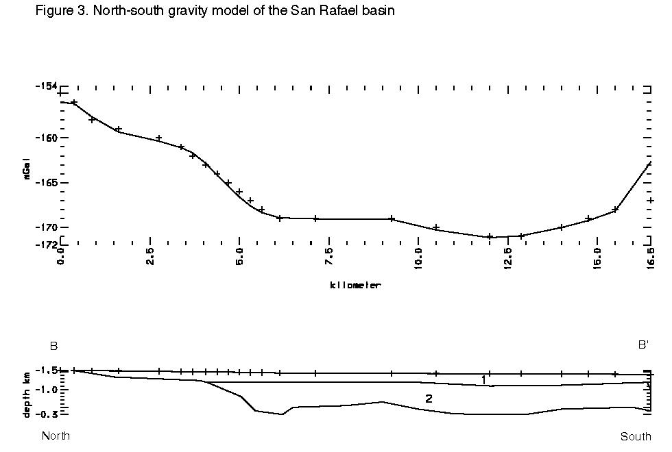
Figure 3 shows that the step model worked fairly well to describe the steep gravity gradient. Body densities are given in Table 6. In reality this gradient is probably due to several small step faults due to its unusual angle and that the bottom of the basin has to come back up slightly to the south of the fault in order to model correctly. Based on the modeling in Figure 3, the thickness of upper basin fill at the deepest portion of the basin is 320 meters and the maximum depth is 1.14 kilometers. It was difficult to model the anomaly properly without an upper basin fill thickness of 320 meters.
Table 6. Map units and densities of bodies used in the forward model of Figure 3.
| Body | density | density contrast | map unit |
| (fig. 3) | (g/cc) | (2.65 g/cc bedrock) | (if abbreviation see Plate 1) |
| 1 | 2.20 | -0.45 | Upper basin fill |
| 2 | 2.32 | -0.33 | Nogales Formation (Lower basin fill) |
The gravity model of the San Rafael basin uses two basin fill units. The lower basin fill unit is probably lower and middle Miocene age and is poorly to moderately well consolidated and is likely to be equivalent to the Nogales formation mapped to the east in the Santa Cruz basin. This lower basin fill unit can be modeled with an average density of 2.32 g/cc. The upper basin fill unit is upper Miocene to lower Pleistocene and is unconsolidated to poorly consolidated. These two basin fill units are overlain by Holocene surficial deposits including alluvium of stream channels, flood plains, and terraces which are unconsolidated overall but locally well indurated. The upper basin fill unit and the thin Holocene surficial deposits are combined into one unit for the purpose of gravity modeling and can be modeled with a density of 2.20 g/cc.
The upper basin fill appears to be thinnest on the western margin of the basin and the lower basin fill is exposed on the northwest margin of the basin. The upper basin fill thickens to the east and south reaching a thickness of over 300 meters. Modeling indicates that it may retain this thickness throughout the central and eastern portion of the basin. The basin has a maximum depth of approximately 1.05 kilometers plus or minus 0.1 kilometers. At least in the southern portion of the basin, it can be modeled as a half-graben faulted on the western margin. The northern portion of the basin is structurally more complex and may have high angle faults on its western, northern, and eastern margin. If the thickness of the upper basin fill based on modeling is accurate, and, if the porosity and permeability are similar to the upper basin fill in the Santa Cruz basin or the western San Pedro basin, the water resources within the upper basin fill aquifer of the San Rafael basin could be significant.
Part 3. Incorporating Earth’s magnetic field data to provide information on basin structure and concealed lithology3.1 Introduction
In order to better understand the structure and concealed lithology of the San Rafael basin, data from the Earth’s magnetic field is used to complement the gravity based study of Part 2. Two types of magnetic field data are used: 1) near ground, closely spaced Earth’s total intensity magnetic field data acquired with a truck-mounted magnetometer and 2) airborne Earth’s total intensity magnetic field data acquired at 1/3 mile spacing.
3.2 Near-ground, closely spaced Earth’s total intensity magnetic field data
Geologic interpretations based on Earth's magnetic field data can benefit by using data that is acquired near ground level and is continuous or closely spaced. Since magnetic fields are dipolar, the magnetic effect due to an object of a given susceptibility falls off as the distance from the observation point to the object cubed. Acquiring data near the ground (near the magnetic sources) maximizes the information content extracted from the Earth's magnetic field.
Magnetic profiles created from near-ground, closely spaced Earth’s total intensity magnetic field data are generally much rougher in appearance than aeromagnetic profile data, even when the latter is flown at low altitude. This rough appearance is a representation of the heterogeneous distribution of sources and their susceptibilities within the volume of rock contributing to the signal acquired by the sensor. This data is useful for precise geologic modeling, depth determination, and in some cases, it can be used to identify lithologies that are concealed by shallow non-magnetic basin fill (Bultman, 1995). Lithologic discrimination is accomplished by either qualitatively or quantitatively defining the texture of the magnetic signal from a given lithology and applying a complex analysis procedure to this data (in the quantitative case).
The Earth’s total intensity magnetic field data used for this study is acquired at intervals of 5 to 15 meters with a truck-mounted proton precession magnetometer. This instrument, originally designed for airborne use, is mounted on a utility vehicle using a retractable boom. The magnetometer sensor is located away from the field generated by the truck, about 5 meters behind the vehicle and about 4 meters above the ground. The proton precession magnetometer has a precision of plus or minus one-hundredth nano- Tesla (nT) and sampling is done at 1 Hertz, rates higher than this are difficult to obtain with a proton precession instrument due to large variations in the magnetic field near ground level. Location data is calculated by dead reckoning along mapped roadways between known points that may be spaced from 100 meters to 2 kilometers. Data are recorded digitally and over 4,000 kilometers of profile data has been obtained in Arizona, New Mexico, and Colorado.
3.3 Discriminating lithology based on near- ground, closely spaced Earth’s total intensity magnetic field data
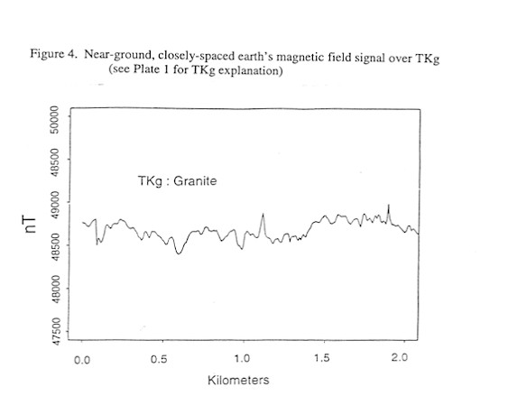
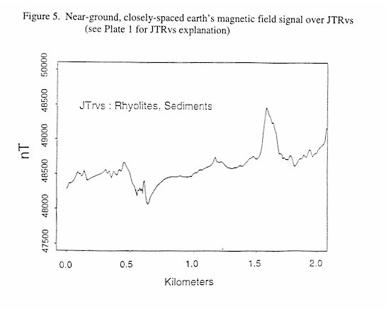
Figures 4 through 9, shown below, display near-ground, closely spaced Earth’s total intensity magnetic field data acquired over different exposed lithologies with identical scaling along both the ordinate and the abscissa. These Figures demonstrate that individual lithologies can display a unique magnetic signature, or texture, and that a wealth of structural information can be available in the data. This texture, defined by the amplitudes and wavelengths of the magnetic signal, is due to the spatial distribution of magnetic sources within a given lithology. While qualitative distinctions can be made and are quite useful, quantitative classification of each texture is ideal.
Geologic and geophysical phenomena manifest themselves over very large ranges of scale. This may indicate that ideas and measures based on fractal geometry can be useful, or may even be necessary, in describing spatial relationships of these phenomena. Since this large range of scales is seen in truck-mounted magnetometer data, and because of observed non-stationarity of the signal and superimposed effects of deep sources, standard statistics alone may not accurately describe the textures contained within these profiles. The fractal nature of the Earth’s total intensity magnetic field is thus used to improve the quantitative textural description of the data.
Fractal scaling has been demonstrated in many geological processes including: porosity measurements derived from neutron density logs; borehole resistivity; density and natural gamma borehole logs; magnetic susceptibility from borehole logs; aeromagnetic profiles;the distribution of faults, fractures, and joints; the sizes and spatial distribution of ore deposits; the topographic shape of the Earth’s surface and in closely spaced total intensity Earth’s magnetic field data (Gettings and Bultman, 1995). The theoretical reasoning behind the fractal nature of the Earth’s magnetic field is thought to be due, at least in part, to a fractal spatial distribution of magnetic sources. Very realistic models of the Earth’s magnetic field have been built by using a fractal distribution of magnetic sources (Gettings and Bultman, 1997). It should be noted that, because the scaling of magnetic field intensity is different from that of position, the Earth’s magnetic field behaves as a self-affine fractal.
A number of textural measures are useful in quantitatively describing the magnetic signature of a given lithology (Bultman and Gettings, 1994). These include the mean and variance of the data, the Euclidean length of the data divided by the distance over which it was acquired, the number of peaks an troughs in the data divided by the distance over which it was acquired, and the fractal dimension. The fractal dimension of the data has been obtained in most cases by two methods that can be used to generate the fractal dimension of self-affine fractals. These are: 1) the rescaled range method (Feder, 1988); and 2) the power spectrum method (Dubuc, 1989). The rescaled range method seems to be the most robust when used with truck-mounted magnetometer data and is the preferred method.
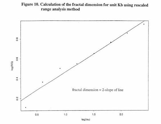
In the rescaled range method, (Feder, 1988), R represents the maximum range of the data in a window of width tau. S is the standard deviation of the data in that window. Windows of varying tau are moved over the entire data set. The logarithm of the ratio R/S is plotted against the logarithm of tau for all tau. The slope of this plot is H, the Hurst exponent, and the fractal dimension, D, of the data is 2-H. It is necessary to be very careful when computing the fractal dimension of self-affine fractals. If the range of the data is such that global fractal dimension of the data is realized, the methodology used will generally display both the fractal dimension and the global dimension (Feder, 1988) of the data, 1. The transition between the self-affine fractal dimension and the global dimension can sometimes be difficult to find and may obscure the true fractal dimension.
3.4 An example of the calculation of the textural measures of the total intensity magnetic field for several exposed lithologies
Examples of the textural measures of near-ground closely spaced Earth's total intensity magnetic field acquired over the exposed lithologies from Figures 4 through 9 are shown in Table 7. The textural measures do a good job discriminating the signals, possibly with the exception of the mean. The variance, and the two of the three measures related to fractal geometry, the data length divided by along ground distance and the fractal dimension, are fairly different for signals that look different.
Table 7. Textural measures of Earth’s total intensity magnetic field for exposed lithologies (see Plate 1 for descriptions of lithologies)
| lithology | mean | variance | Data len./ | # of peaks/ | D |
| (nT) | x- length | x- length | |||
| TKg | 48738.4 | 17107.0 | 3459.3 | 21.6 | 1.86 |
| JTrvs | 48516.7 | 81491.8 | 3492.9 | 17.8 | 1.83 |
| TKvs | 48722.6 | 13810.5 | 3670.1 | 16.9 | 1.73 |
| Yg | 48620.3 | 2917.6 | 959.1 | 19.0 | 1.70 |
| Pzl | 48426.2 | 3186.2 | 1645.3 | 19.0 | 1.68 |
| Kb | 48559.2 | 27580.6 | 1395.7 | 15.5 | 1.64 |
The variance is correlated to deep sources, that is, large anomalies in the observed data. This may or may not be characteristic of a given lithology. The measures related to fractal geometry do a good job describing texture. They are less correlated with large anomalies and tend to represent textural differences in the data better. Observations with higher fractal dimension will generally represent noisy high amplitude data from a very magnetic source lithology.
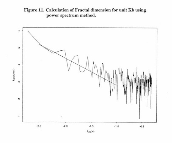
Examples of the plots used to calculate fractal dimension are shown in figures 10 and 11. Figure 10 shows the log(R/S) vs. log(tau) plot used to find the Hurst exponent (H) of the rescaled range method. The fractal dimension is equal to 2-H in the rescaled range method. Based on Figure 10, the fractal dimension of Kb is 1.64. Figure 11 shows the results of the power spectra method. This graph plots log(power) vs. log(w) (where w is frequency). In this method the transition from local to global fractal dimension can be seen at log(w) equal to about –1.0, or approximately a wavelength of 0.37. The fractal dimension is derived from the slope of the data in the high frequency portion of the curve (see Dubuc, 1989) that represent the local fractal dimension. Based on Figure 11, the fractal dimension of Kb is 1.68, in general agreement with that fractal dimension calculated from the rescaled range method. This example has been presented to indicate that the calculation of the fractal dimension for a self-affine fractal is not an exact science. Most methods are based on the slopes of lines acquired from data that are not linear and only cover a certain range of wavelengths, as can be seen in figures 10 and 11. The calculations of fractal dimension are estimates, probably good only to two significant Figures although three significant Figures will be presented in this report.
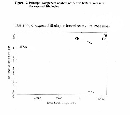
A principal components analysis of the textural measures was done so that all 5 textural measures could be summarized and plotted in 2 dimensions (Figure 12). Examination of the eigenvalues and the textural measures shows that the first principal component is highly dependent on the variance measure. The second principal component is highly dependent on the fractal dimension. As Figure 12 shows, the textural measures seem to differentiate lithologies that appear texturally different (JTRvs and Pzl) and group together lithologies that are similar (Yg and Pzl).
3.5 Estimating concealed lithology
Total intensity magnetic field data acquired over shallow Cenozoic basin fill contains a signal component from the basin fill and a signal component from the underlying bedrock lithology in most cases. Both components are fractal or multifractal and combine to form a multifractal signal. If the "roughness" or amplitude of the signal component from the concealed lithology dominates the texture of the total magnetic signal acquired over basin fill (the target signal), it is generally possible to narrow the choices of potential concealed lithologies to a list of candidate lithologies. Many lithologies whose magnetic signature would not show through the basin sediments (those with very low amplitudes) can be eliminated. In limited cases, quantitative techniques can be used to identify a lithology if the textural measures of each of the candidate lithologies are very different (Bultman and Gettings, 1994). In this section we will test whether we can distinguish between concealed lithologies whose magnetic signatures where exposed are similar. The importance of integrating all geologic constraints when doing this type of analysis can not be overemphasized.
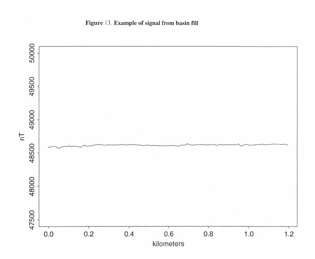
In most basins in southern Arizona the basin fill alone is almost non- magnetic, its magnetic signal has only a small amplitude of about plus or minus 20 to 30 nT from its mean (Figure 13). If a lithology with a magnetic signature that has a large amplitude (plus or minus 100 nT or more from its mean) is concealed below the basin sediment fill, this amplitude will show through the basin fill provided the concealed lithology is not buried too deeply. Concealed lithologies with small amplitude signals will not be detectable through basin fill and can be eliminated as candidate lithologies when a large amplitude signal is observed in truck-mounted magnetometer data acquired over basin fill.
A method for quantitatively identifying a lithology whose magnetic signal is detectable through basin sediments is outlined here. The method begins with the selection of several candidate lithologies based on the magnetic signature of their outcrop and the geological relationships within the region in question. The process of upward continuing a magnetic signal will be used to lower the observed signal from candidate lithologies to a depth equal to their burial under basin sediment. This process smoothes the signal and lowers its amplitude as shown in Figure 14. The signal from the basin fill is obtained by a high-pass filter that removes all signals from below the estimated depth of fill at the region in question. This basin fill signal will then be added to the signal from the upward continued candidate lithology to form a synthetic signal. The synthetic signal will then be compared to the target signal acquired over basin fill.
It is hoped that many of the textural measures based on fractal geometry will retain their value through the upward continuation process and allow the candidate concealed lthologies to be discriminated. Previous work has shown that the fractal dimension of synthetic signals can be used to discriminated low amplitude concealed lithologies with high amplitude concealed (Bultman and Gettings, 1994).
An example of this procedure is shown in Figures 15 and 16. The magnetic field signal acquired over exposed candidate lithologies is upward continued by an amount equal to the estimated depth of burial of the concealed lithology. This is shown in the upper left portion Figure 15, here the signal over the candidate lithology was upward continued 50 meters. The signal due to the upper 50 meters of basin sediment is shown in the upper right portion of Figure 15 with an expanded scale on the ordinate. This is obtained by upward continuing a target signal by an amount equal to the estimated depth of burial of the concealed lithology and subtracting it from the original signal. It is important to use the basin signal at the location of the target signal in order to account for the magnetic texture of the proper facies of basin sediment that lie above the concealed lithology. The upward continued candidate lithology and the signal from the upper 50 meters of basin fill are added to form a synthetic signal that is shown in the lower right portion of Figure 15. This signal is compared to the actual signal through the use of the textural measures. This process is repeated for all candidate lithologies.
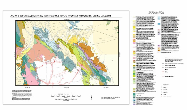
In the San Rafael basin two test areas have been chosen in order to apply this methodology. The first is on the southwest margin of the basin and is labeled site 1 on Plate 7. The second is on the northern margin of the basin and is labeled site 2 on Plate 7. The depth to bedrock is estimated to be shallow in these area (50 and 100 meters respectively) and the magnetic signal acquired in these areas contains a large amplitude component, part of which is believed to come from the concealed bedrock. Both areas are also very close to the basin margin, and it is likely that the lithology at the basin margin is found concealed at each site.
Click here to view Plate 7 at scale
Click here to go to the Postscript archive for Plate 7
Test site 1 occurs just beyond the basin-bedrock contact with Jurassic- Triassic volcanic and sedimentary rocks. It is likely that these volcanic rocks continue into the basin for some distance to the east, at least until a high angle basin fault is found. The target signal over the basin is shown in Figure 16. It has a very high amplitude and looks unlike the signal from the basin sediments of Figure 13. This signal most likely contains information from the lithology concealed beneath the basin fill. The large amplitude of the target signal and the local geology indicates that the candidate unknown lithologies are TKg, JTRvs, and TKvs. These candidate lithologies are processed as described above and their textural meaures are shown in Table 8. Along with the textural measures of the tagret signal and the basin fill.
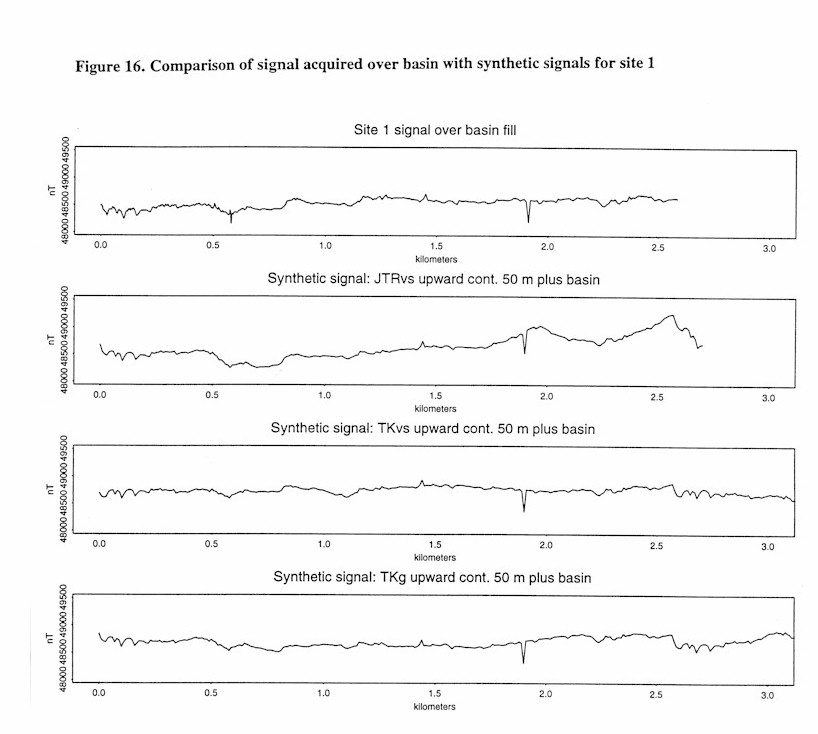
Based on Table 8, there is no clear-cut selection as to what is the concealed lithology. The signal for the JTRvs candidate lithology was acquired just to the north of the area and it has a large variance. This variance is due at least in part to large structures and probably invalidates and comparisons based on the variance measure. The data length divided by along road length (x-length) and the number of peaks divided by x-length are similar between the the candidate lithologies, but not really the unknown. The fractal dimension also follows this pattern. The precision of measuring fractal dimension is probably only 0.1, note that this would not allow any distinctions to be made based on the fractal dimension in this data except for the basin fill itself.
Table 8. Textural measures of Earth’s total intensity magnetic field for concealed Lithology site test 1 (see Plate 7 for descriptions of unit and location of target signal)
| map unit | mean | variance | Data len./ | # of peaks/ | Fractal |
| x-length | x - length (for all data) | dimension (for all data) | |||
| target signal | 48491 | 11174 | 3052.9 | 39.0 | 1.82 |
| basin fill alone | 0 | 2082 | 2129.2 | 22.8 | 1.58 |
| TKg up 50m + basin | 48735 | 10753 | 2208.0 | 22.0 | 1.90 |
| JTrvs up 50m + basin | 48635 | 49053 | 2513.3 | 18.9 | 1.90 |
| TKvs up 50m + basin | 48721 | 5527 | 2173.5 | 21.8 | 1.87 |
Test site 2 occurs in the northern portion of the basin south of the large outcrop of TKvs. In this area it is assumed that the TKvs unit continues to the south under the basin sediments. Figure 17 shows th ecomparison of siganals. Table 9 displays the textural measures. In this region the textural measures do not allow for the determination of any concealed lithology. While the measures are more similar to the target signal measures than in site one, it is still impossible to differentiate which lithology matches the target signal.
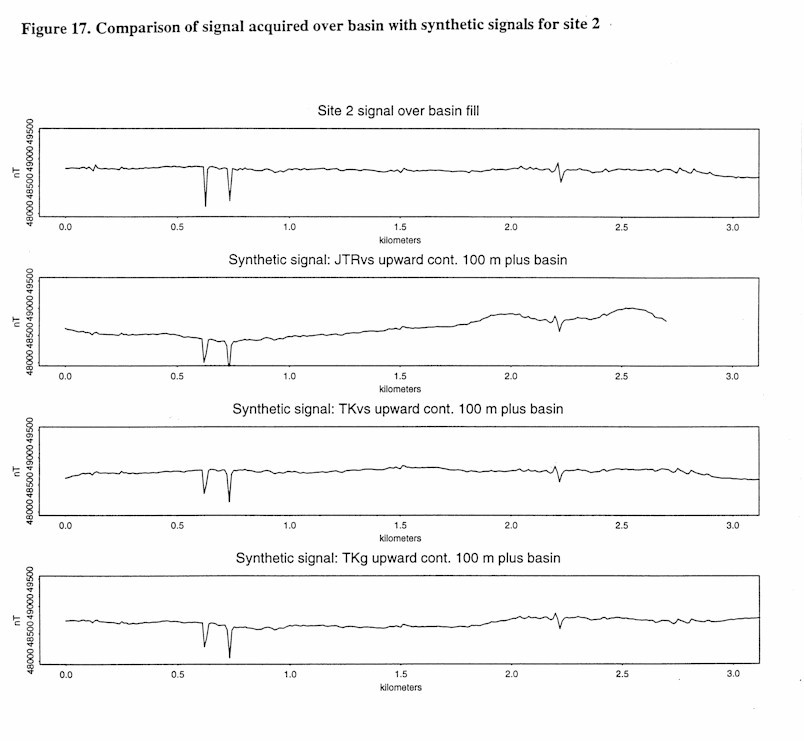
Table 9. Textural measures of Earth’s total intensity magnetic field for concealed lithology site test 2
(see Plate 7 for descriptions of map unit and location of target signal)
| map unit | mean | variance | Data len./ | # of peaks/ | Fractal |
| x-length | x-length | dimension | |||
| target signal | 48827 | 9108 | 2039.6 | 21.3 | 1.71 |
| basin fill alone | 0 | 2481 | 1561.8 | 22.1 | 1.59 |
| TKvs up 100m + basin | 48720 | 4310 | 1767.1 | 23.9 | 1.66 |
| JTRvs up 100m + basin | 48632 | 34355 | 1961.3 | 18.9 | 1.67 |
| TKg up 100m + basin | 48735 | 8431 | 1600.9 | 22.0 | 1.74 |
3.6 Problems with the quantitative estimation of concealed lithology
It is obvious from the results of test sites 1 and 2 that the method outlined here for the estimation of concealed lithology does not work very well when candidate lithologies all have rough textured, high amplitude signals. There a number of potential problems that contribute to the inability of the textural measures to consistently predict concealed lithology. Facies changes in the candidate lithology (map units) or the concealed lithology may mean that the magnetic signature of a given lithology can change over only a short distance. Most map units in the United States are based on time- stratigraphic mapping practices and may contain several separate lithologic units.
Most near-ground closely spaced Earth’s magnetic field data is acquired while driving about 20 miles per hour. This works out to approximately 1 data point every 10 meters. In fact, data are interpolated to 10 meter spacing for input into the Fourier transform routine which is needed for upward continuation. Data at spacing of 10 meters may not be sufficient to capture the fractal geometry related properties of some lithologies and/or basin sediments. With the acquisition of a new magnetometer, data acquired after 1998 will be sampled approximately every meter.
Both the synthetic signal and the unknown signal are multifractal. They contain components from bedrock, or possible bedrock, and basin fill. What the multifractal relationships have on the textural measures is a complex issue and more research must be done to understand their effects.
Due to these problems, the method outlined above for identifying concealed lithology and the observations based on it at this time must be considered very preliminary. Past work has shown that this method can discriminate low amplitude smooth signals from high amplitude rough signals, but to a large degree this can be done visually.
3.7 Structural information from truck-mounted magnetometer data
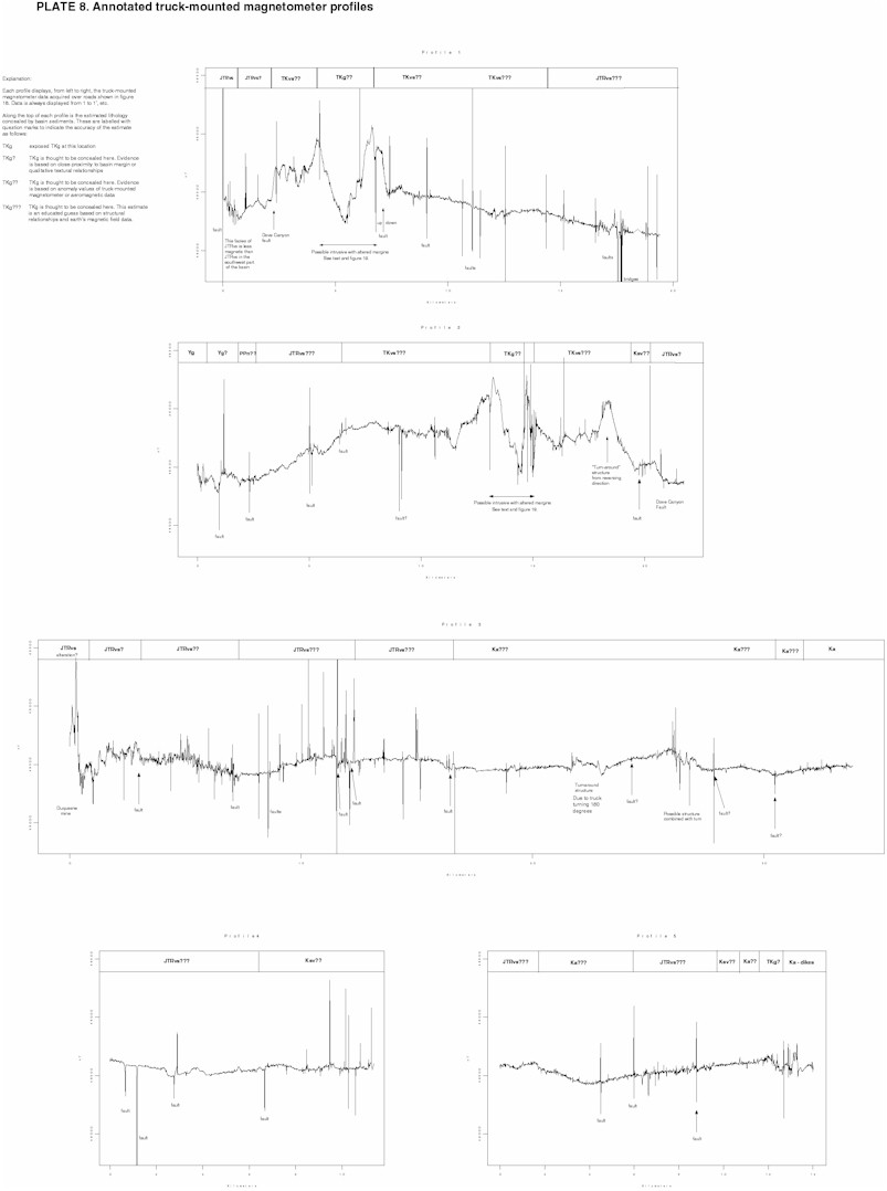
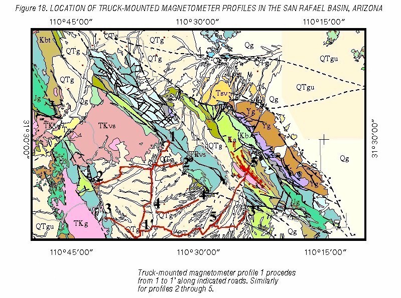
Plate 8 displays most of the truck-mounted magnetometer data that has been acquired over the San Rafael Valley. The data is displayed as 5 profiles that are keyed to the map in Figure 18. Profile 1 extends from 1 to 1’ on Figure 18 and likewise for each of the other profiles. The near- ground closely spaced data has had cultural features removed. The data is useful for observing textures that may contain information on very magnetic concealed lithologies, looking at its overall value (at scales of 100 of meters or more) to ascertain whether the bedrock has a high or low susceptibility (this concept will also be applied using aeromagetic data in the next section), and especially for finding faults. There are many reasons that faults may show up in near-ground closely spaced magnetic profiles, these include contrasting lithology (the fault may separate lithologies or facies of a map unit), fault gouge, and fault related mineralization. Many of the faults are short wavelength and high amplitude, indicating that they are shallow features. When this is the case, the faults are only forced into the concealed bedrock if their is some indication from the aeromagnetic data that they may occur in the bedrock. This data points out that truck-mounted magnetometer data is a good way to find faults in the basin fill and concealed faults.
Click here for full scale Plate 8 (large file)
Click here to go to the Postscript archive for Plate 8
Profile 1 through 5 on Plate 8 are annotated with structural features. Along the top of each profile, the concealed lithology is estimated. The accuracy of these estimates varies, and each estimate is keyed to the accuracy description at the top left of the Plate. The estimates of concealed lithology presented here are the best estimates that could be made at the time this report was written based on current data, knowledge, and procedures. They are qualitative estimates based on geologic principals.
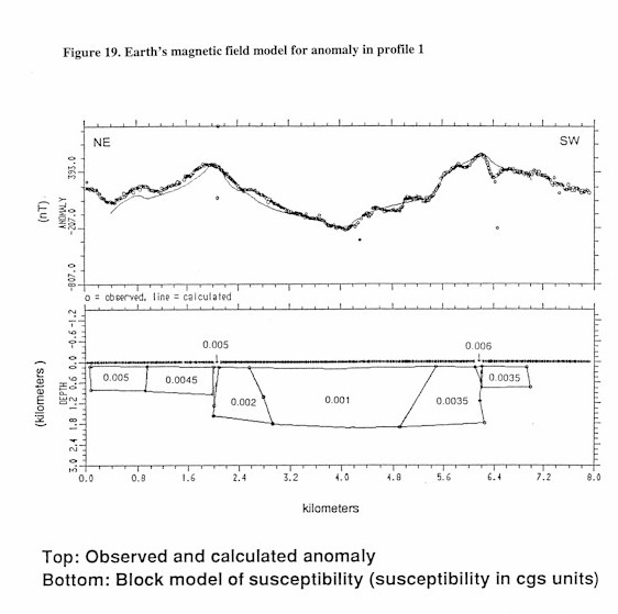
Profile 1 begins in map unit JTRvs (volcanic sediments) on the north margin of the basin. The JTRvs map unit in this region seems to be less magnetic than in map units found to the west and south. The profile enters the basin and the low value and smooth texture indicates that JTRvs probably continues concealed here. The Dove canyon fault is crossed at the 2.3 kilometer mark. This does not seem to affect the basin depth, but the lithology changes to a very magnetic unit with a rough texture. Given the geologic relationships in this region, it is assumed to be TKvs (Laramide volcanic sediments, mostly andesite) which outcrops just to the north. The profile then encounters a major structure that was interesting enough that the magnetic signal over this structure was modeled. Figure 19 displays this model which can be summarized as an intrusive stock (Tkg) surrounded by an alteration halo, possibly skarn, buried under about 100 meters of basin fill. This feature can not be seen in any of the published magnetic maps of the region. Once past the structure, the profile crosses some major fault blocks (near km. 7) that coincide with the faults modeled in Figure 3. Here, the bedrock falls away to about 500 meters depth. As the profile continues, the basin becomes deeper, crosses several faults, probably transitions into less magnetic rocks, and encounters structural features near the 17 to 18 kilometer mark.
Profile 2 displays a roughly west to east truck-mounted magnetometer profile across the northern San Rafael Valley. The entire profile, except about one kilometer on the west end, was acquired over basin fill. This profile starts out in the altered rocks near the Mowry mine then enters the basin fill from map unit Yg (Pre-Cambrian granite) where the depth of sediments stays fairly shallow. The concealed lithology probably stays the same or may include some Paleozoic sediments that are found exposed nearby. The basin stays shallow until it encounters the fault at 5 kilometers on the profile. Here it deepens rapidly to about 500 meters, then shallows again. The concealed lithology in this region can only be guessed at because there is a lot of structural information in the signal. The profile enters TKvs near the 7 kilometer mark (based observationally on the texture of the magnetic signal and the fact the TKvs is exposed just to the north). It stays in this unit, crossing many faults and structures, until the 19 kilometer mark where it enters Ksv (Cretaceous volcanic and sedimentary rocks-based on local geology and observed magnetic signal). At about 20 kilometers, the profile crosses the Dove Canyon fault and enters what is probably JTRvs.
Profile 3 begins in JTRvs in the southwest part of the San Rafael Valley. The profile moves over several blocks of JTRvs (based on local geology and observed magnetic texture) until it encounters the main basin bounding fault at about 7.5 kilometers. This location matches the faults seen in the gravity based model of Figure 3. The rough appearance of the truck-mounted magnetometer signal over this region indicates that the basin may be more shallow than predicted by gravity modeling, especially in the models built from the gravity profile of Figure 2. By making body 6, Figure 2, less dense, the model fits as well as before, yet allows for a fairly shallow part of the basin in this area. Figure 20 displays a new gravity model based on this change which is probably more accurate than the model shown in Figure 2. The density of body was changed from 2.75 g/cc to 2.62 g/cc, a number that works well for the map unit JTRvs. The new density model for each body in Figure 20 is shown in Table 10. The fault at 7.5 kilometers in profile 3, Plate 8, then has more offset that shown in Figure 2. This is consistent with the truck-mounted magnetometer data.
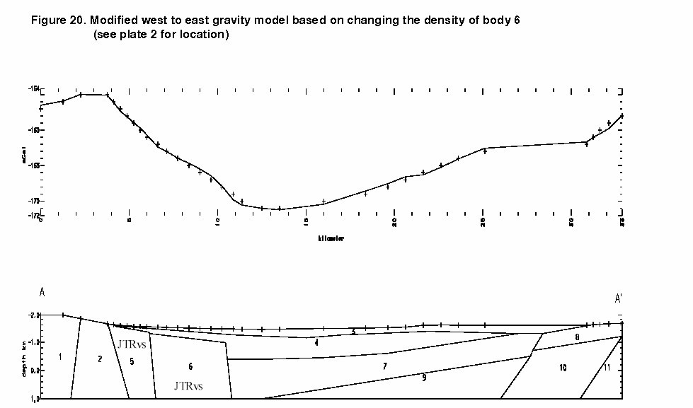
Table 10. Map units and densities of bodies used in the new forward model of Figure 20.
Body density density cont. map unit (? = Inferred) (fig. 20) (g/cc) (2.65 g/cc ) (if abbreviation see Plate 1) 1 2.66 0.01 TKg 2 2.70 0.05 PPn (likely a dolomite facies) 3 2.20 -0.45 Upper basin fill 4 2.32 -0.33 Nogales Formation-Lower basin fill 5 2.65 0.00 JTRvs 6 2.62 -0.03 JTRvs? 7 2.65 0.00 Kb? (Bisbee Formation) 8 2.50 -0.15 Ka 9 2.75 0.10 PPn? (likely a dolomite facies) 10 2.60 -0.05 Ka? 11 2.75 0.10 PPn? (likely a dolomite facies)
Profile 3 continues by crossing a number of structures between kilometer 8 and 12. The basin is deep and, except where a fault is crossed, only basin fill textures can be seen in the profile. The prominent feature at kilometer 11 is a bridge over the Santa Cruz River, but this also seems to coincide with a structure. At kilometer 17, there seems to be a quieting of the magnetic signal from the truck-mounted magnetometer, probably indicating a different facies of basin fill. The signal remains quiet until the basin shallows near the 30 kilometer mark. It is assumed that the concealed lithology in this area is Ka, which is found close by at the basin margin.
Profile 4 is in the east central portion of the basin. This profile provides locations of several concealed faults and shows the possible fault boundary between the deeper bedrock and Ksv. A number of faults are visible at the eastern side of this profile.
Profile 5 is on the eastern margin of the basin. It begins in a fairly deep portion of the basin where no magnetic texture based lithologic distinctions could be made. Based on the long wavelength features seen in profile 5, the bedrock is thought to be JTRvs from 0 to 1.8 kilometers and Ka from 1.8 to 6 kilometers. At kilometer 6, a fault seems to separate lithologies. A magnetic lithology with a rough texture lies under the profile from 6 to 9.5 kilometers, this is thought to be JTRvs due to the JTRvs outcrops to the north and south. At the 9.5 kilometer mark, there are textural changes that may indicate corresponding lithologic changes to Ksv, then to Ka, and finally to TKg. These concealed lithologies are well constrained in this narrow valley.
3.8 Airborne Earth’s magnetic field data
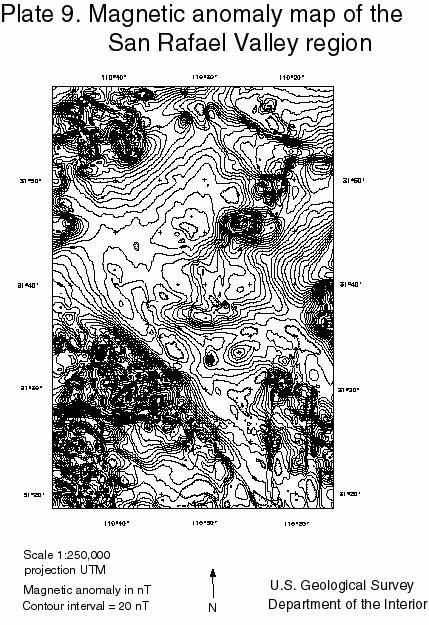
The airborne Earth’s magnetic field data used in this report was acquired by Geometrics in 1975 as a joint venture for several mining companies. The data was acquired at an altitude of 750 feet above the ground with a 0.33 mile traverse line spacing. This data was gridded at a 0.5 kilometer grid cell size and contoured with a minimum curvature routine. The contour interval was chosen to be 20 nT in order to discriminate features in the basin. At this contour interval, contours in the ranges quickly become stacked on top of each other and the contouring algorithm thus fails. The contour map of the magnetic anomaly data is displayed in Plate 9. This Plate has been presented at a scale of 1:250,000 to comply with stipulations made by Pearson, deRidder and Johnson, the present day owners of the data set. This makes it very hard to see many of the features that have been incorporated into the interpretation of this section and Part 4. The principal direction of flight lines was east-west. There are north-south tie lines at 5 mile intervals and it can be seen that these tie lines have not been completely reduced. However, the data over the San Rafael basin is good.
Several northeast trending faults can been seen cutting the Canelo Hills in this aeromagnetic data (when displayed at 1:125,000 or smaller scales). These faults seem to represent a down stepping of the magnetic source material from northwest to southeast in the Canelo Hills. Also, a sharp magnetic anomaly, labeled as a possible intrusive in Plate 8, Profile 1, can be seen in this aeromagnetic data. This anomaly is modeled as an concealed intrusive in figure 19. In the aeromagnetic data, it appears that part of the anomaly may be due to a reversed magnetic field in part or all of the magnetic source rock. This anomaly, near the northern end of the San Rafael basin, is northeast trending and about 1.25 miles long by 1 mile wide. It lies directly on one of the northeast trending faults visible in the aeromagnetic data.
Aeromagnetic data is much better suited to detecting deeper magnetic features that truck-mounted magnetometer data and this data will be used for that purpose. Units that are more magnetic will tend to keep the magnetic field high and vica-versa. By combining the locations of faults based on the truck-mounted magnetometer data, with the local value of the field from this aeromagnetic data, inferences about concealed lithology can be made. This is done in Part 4.
Click here to go to the Postscript archive for Plate 9
Part 4. Concealed structure and lithology in the San Rafael basin4.1 Putting it all together
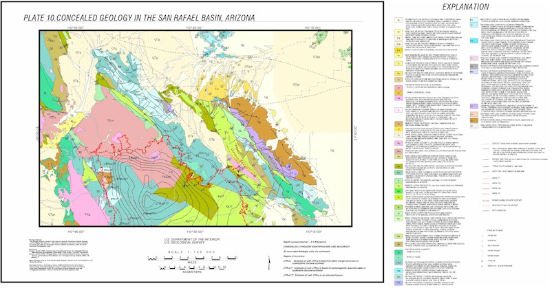
With basin geometry based primarily on gravity data, basin structure and concealed lithology based on near-ground closely spaced Earth’s magnetic field data, and deep basin features based on 1/3 mile spaced aeromagnetic data, we are now ready to put it all together to form a map of the concealed lithology of the San Rafael basin. That map is displayed in Plate 10.
Click here to view Plate 10 at scale
Click here to go to the Postscript archive for Plate 10
The concealed geology map was constructed as follows. Depth to bedrock contours are taken directly from Plate 6. Along the basin margin, exposed faults are extended and, if possible correlated with faults that occur in the truck- mounted magnetometer data. Lithologies (map units) are extended out from the basin margin until there is some indication of change, generally a fault and/or a change in magnetic texture in the near-ground closely spaced Earth’s magnetic field data. Fault data, near-ground closely spaced Earth’s magnetic field data, and the aeromagnetic data of Plate 9 are used to identify lithology and structure in the deeper portions of the basin. In general, a magnetic lithology is placed where the Earth’s magnetic field anomaly is high in Plate 9 and a non-magnetic lithology is used if it is low. All possible geologic constraints are used when doing this. The intrusive visible in Plate 8, Profile 1, and modeled in Figure 19 is displayed as a concealed Laramide granitic intrusive (TKg) in the northern portion of the basin.
Plate 10 presents the concealed lithology with three types of accuracy. If the concealed lithology was estimated by it being exposed at the basin margin, and/or by the textural properties of near-ground closely spaced Earth’s magnetic field data, and by considering the local geology, it is displayed with one question mark indicating that that is the best estimate of the three. If the concealed lithology is estimated based on the magnitude of the Earth’s magnetic field data and by considering the local geology, it is displayed with two question marks. This indicates an intermediate level of confidence. If the estimation of the concealed lithology was an educated guess based on local geology and, possibly, on the magnitude of the Earth’s magnetic field data, it is assigned three question marks indicating it has the lowest level of confidence.
Many things can be learned by integrating this data. The locations of faults is probably accurate. The concealed lithologies are probably accurate near the basin margin, In other areas only drilling will tell. Based on the aeromagnetic map of Plate 9, the magnetic anomaly displayed on Plate 8 profile one and modeled in Figure 19 may dip to the southwest. The basin can be modeled as an asymmetric graben, with its major fault on the western margin of the basin, in the southern part of this study area. The northern part of the basin appears to have high-angle normal faults on the west, north, and east side.
A mineral resource potential similar to the major districts of the Patagonia Mountains exists in the western part of the basin. The concealed lithology data, depth to bedrock information, and fault information are all important keys to this potential. Economics dictates the depth at which these potential deposits become minable, but there is a large area in this region that is less than 500 meters deep. The northern margin of the basin also holds a great deal of mineral resource potential. A major porphyry copper deposit exists just to the northwest of the basin and the anomaly modeled in Figure 19 indicates that it is possible one may exist concealed by sediments at the location indicated at map unit TKg in Plate 10.

![]() U.S. Department of the Interior |
U.S. Geological Survey
U.S. Department of the Interior |
U.S. Geological Survey
URL: http://pubsdata.usgs.gov/pubs/of/1999/0399/intro.html
Page Contact Information: GS Pubs Web Contact
Page Last Modified: Wednesday, 07-Dec-2016 17:51:10 EST

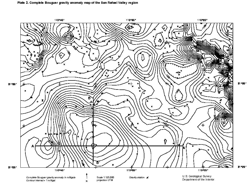