
Open-File Report 00-138, Online version 1.0
Depth to bedrock in the Upper
San Pedro Valley, Cochise County, southeastern Arizona
By Mark E. Gettings and
Brenda B. Houser1
This report is only available on the web
This report is preliminary and has not been reviewed for conformity
with U.S. Geological Survey editorial standards or with the North American
Stratigraphic Code. Any use of trade, firm, or product names is for descriptive
purposes only and does not imply endorsement by the U.S. Government.
U.S. DEPARTMENT OF THE INTERIOR
U.S. GEOLOGICAL SURVEY
1U.S. Geological Survey, Southwest
Field Office, 520 N. Park Ave., Rm. 355, Tucson, Arizona, 85719
Contents
Estimation of basin geometry from the geologic and geophysical data
Separation of the basin gravity anomaly
Estimation of depth to bedrock
Estimation of thickness of basin fill
Figures
Figure 1. Location map of study area
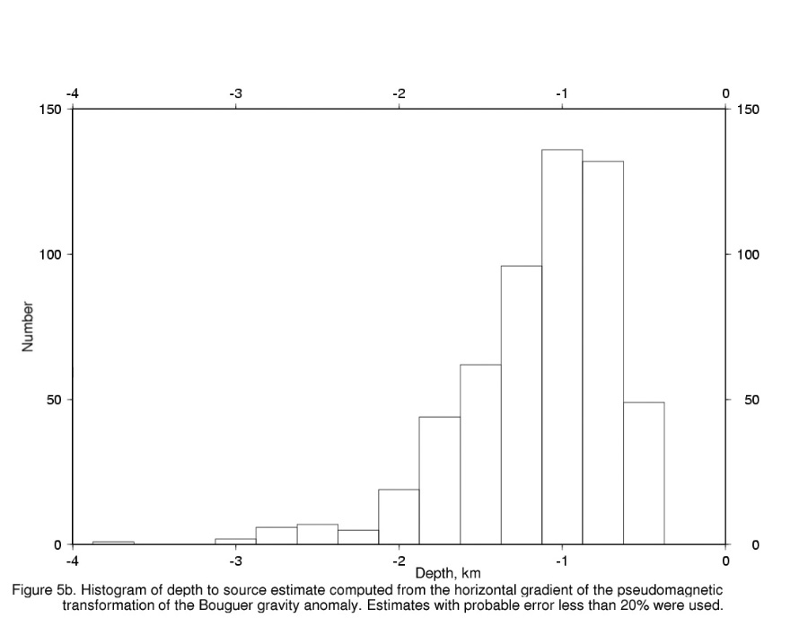
Figure 5b. Histogram of depth to source estimates computed from the horizontal gradients of the pseudomagnetic transformation of the Bouguer gravity anomaly.
Figure 7. Density contrast function relative to bedrock adopted for this study
Plates
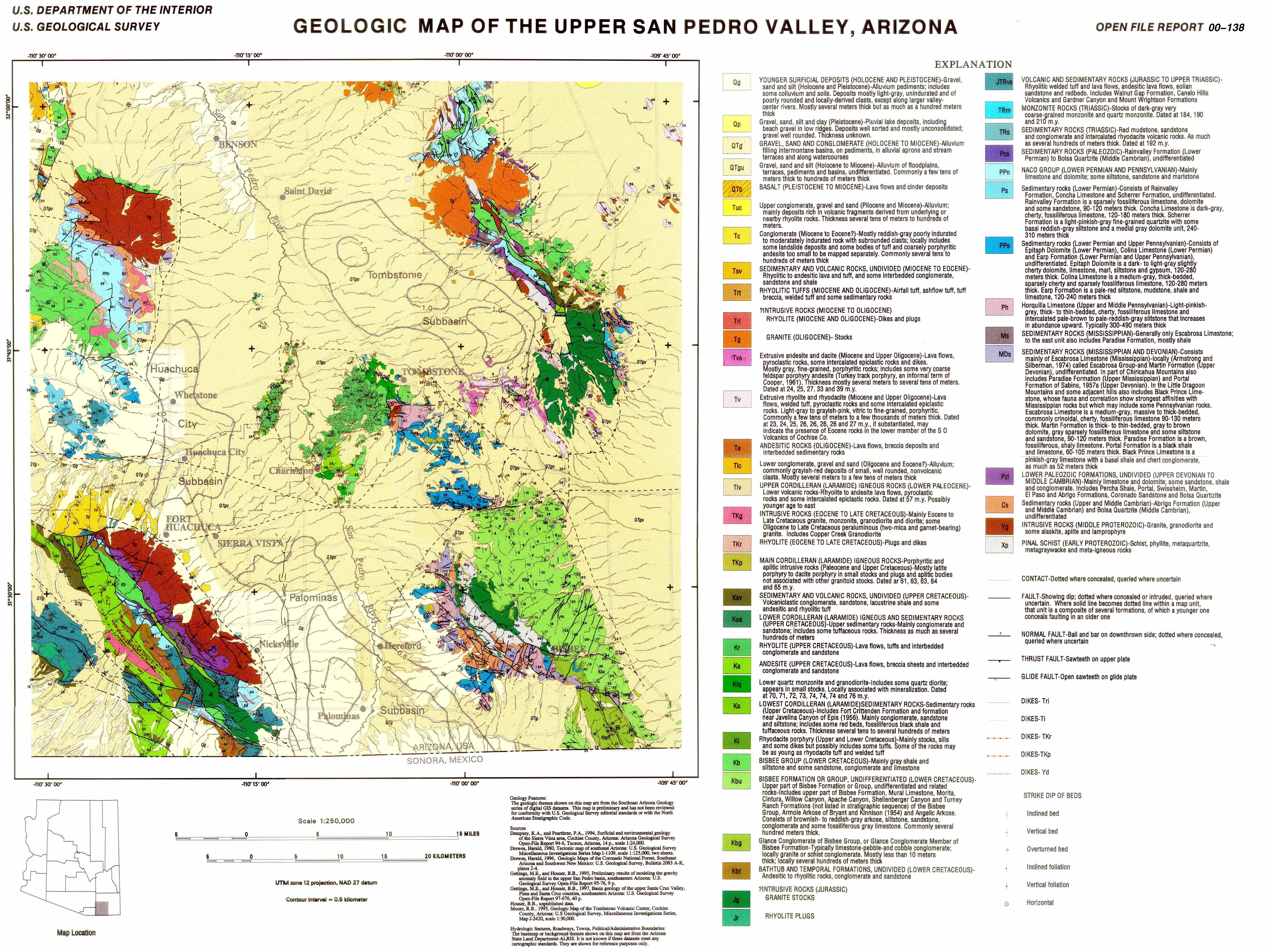
Plate 1. Generalized geologic map of upper San Pedro basin, southeastern Arizona.
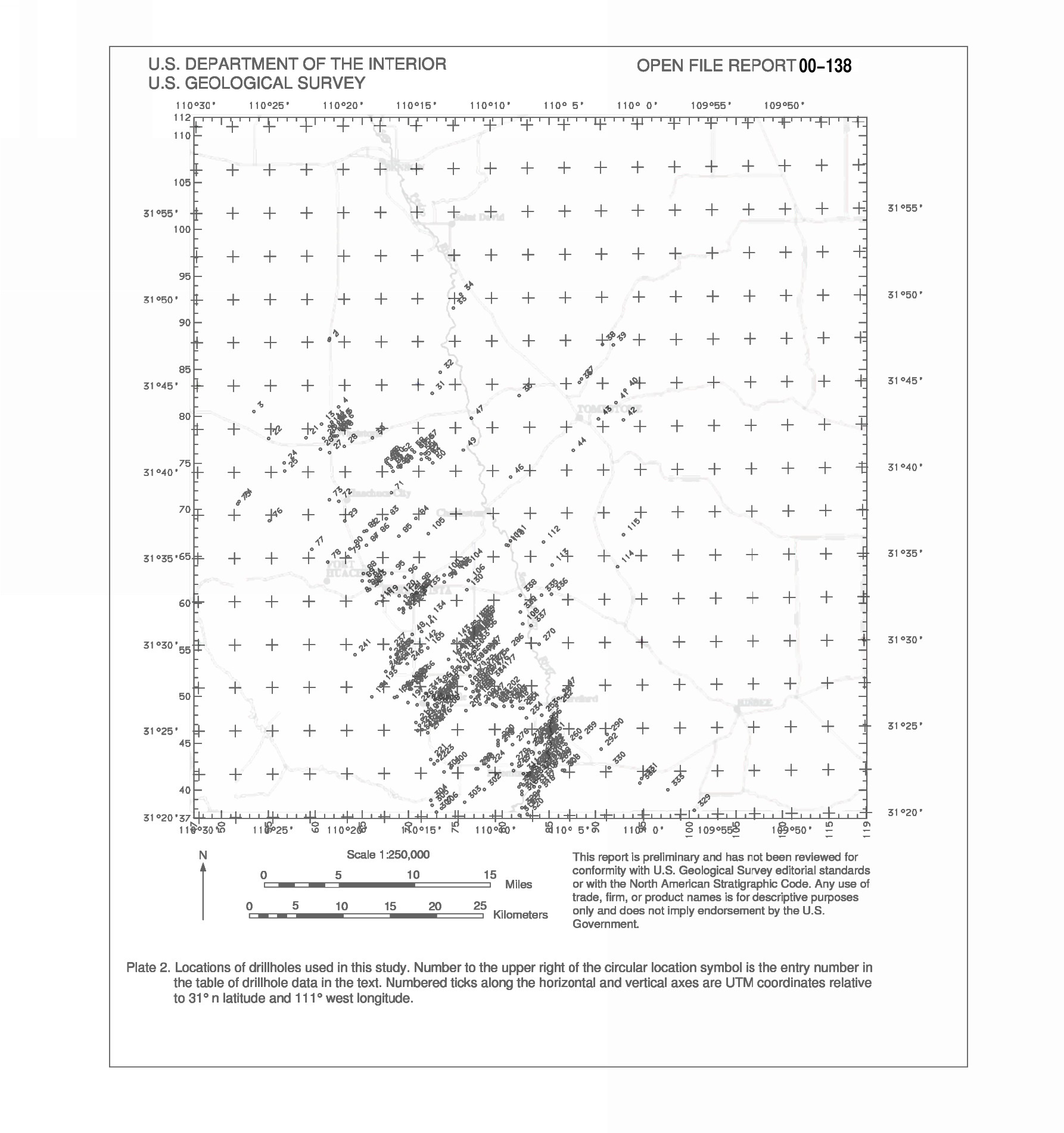
Plate 2. Map showing the location of wells used in this study.
Plate 3. Complete Bouguer gravity anomaly map, upper San Pedro basin, southeastern Arizona .
Plate 5. Residual gravity anomaly map, upper San Pedro basin, southeastern Arizona.
Animations
Tables
Table 1. Log of Phillips Petroleum #A-1, Huachuca State
Table 3. Summary statistics for computed depths to source from the Bouguer gravity anomaly dataset.
Table 4. Density versus depth functions for basin fill, Pantano? Formation, and bedrock.
Appendix 4. Principal facts for the 1,521 gravity stations used in this study.
Appendix 6. Well numbering system.
The thickness, distribution, and character of alluvial sediments that were deposited in the structural subbasins of the upper San Pedro basin in southeastern Arizona during the late Cenozoic provide important constraints on ground-water availability of the area. Two sedimentary units are recognized; the Oligocene and Miocene Pantano(?) Formation and an unnamed upper Miocene through lower Pleistocene unit termed basin fill.
The complete Bouguer gravity anomaly map shows that there are three major structural subbasins in the upper San Pedro basin north of the international border with Mexico. The Tombstone subbasin is north of Tombstone, and two more are located north and south of Sierra Vista, respectively. This report concentrates on the two subbasins north and south of Sierra Vista. The northern subbasin (termed the Huachuca City subbasin) extends from east of Huachuca City to northeast of Whetstone, and the southern subbasin (termed the Palominas subbasin) extends southward from a line between Nicksville and Hereford to the border. The locations and shapes of these subbasins, thickness of basin fill, and depth to bedrock were estimated using a procedure involving interpolation of (1) the density functions derived in this study, (2) stratigraphic data from water wells, and (3) a residual gravity anomaly grid obtained by subtracting the gravity effects of the bedrock ranges bordering the basin from the complete Bouguer gravity anomaly.
This procedure indicates that the subbasins are shallow and contain significant thicknesses of the Pantano(?) Formation in addition to the overlying younger basin fill. The maximum depth to bedrock is about 1,700 m in the Palominas subbasin and 800m in the Huachuca City subbasin; the basin-fill unit occupies the upper 250-350 m in general with local thickenings exceeding 1,000 m in the Palominas subbasin. An east-west trending buried bedrock high beneath Fort Huachuca, Sierra Vista, and Charleston separates the subbasins. The depth to bedrock over this high is 200-500 m and the basin-fill unit ranges from 100 to 200 m thick there. A number of previously unrecognized faults were identified and the lengths of some of the known faults were extended based on reconnaissance geologic mapping, study of driller's logs, interpretation of aerial photographs and thematic mapper satellite images, and inspection of contoured gravity and aeromagnetic anomaly data. Many faults that segment the main San Pedro basin and shape the boundaries of the subbasins are apparently pre-existing faults that have been reactivated by Basin and Range extension.
The San Pedro River, which has its headwaters
in Mexico near Cananea, flows generally northward through the study area
to its confluence with the Gila River at Winkelman, Arizona. This
report addresses the three-dimensional shape of the subbasins that comprise
the 75-km-long reach of the upper San Pedro River Valley from the international
border with Mexico to Benson, Arizona (throughout this report, a larger
version of the figure can be obtained by clicking on the link to the figure,
for example, fig.
1).

Increased ground-water usage due to population growth in the upper San Pedro Valley has the potential to exceed the available ground water of the area in the future, to the extent that perennial flow in the San Pedro River will be affected. Federal, state and local land-use planners need to know the location, thickness, depth, and estimated yield and quality of the ground-water aquifers in the valley. Unfortunately, there is little direct information about the thickness and depth of the aquifers in the valley because few deep wells to bedrock have been drilled. The objective of this study is to use a combination of geologic and geophysical methods to model the shapes and locations of the subbasins that make up the upper San Pedro basin and to estimate the thickness of better consolidated Pantano(?) Formation sediments (poor aquifers) relative to less consolidated overlying basin-fill sediments (better aquifers) in the subbasins.
The upper San Pedro River Valley is in the southern Basin and Range Province of southeastern Arizona and northern Sonora. This terrain of alternating fault-bounded linear mountain ranges and sediment-filled basins began to form about 17 Ma in southeastern Arizona as the result of dominantly east-northeast/west-southwest directed crustal extension. The topography of the basins and ranges in this part of the province has a zigzag northeast and northwest pattern that may be a result of movement along west-northwest-trending Mesozoic faults that were reactivated by the Miocene extension.
The geologic map of the upper San Pedro Valley (plate 1) is part of a digital geologic database created by digitizing the maps of Drewes (1980, 1996) at a scale of 1:125,000. Additional data were then added from Dempsey and Pearthree (1994), Gettings and Houser (1995, 1997), Moore (1993), and from fieldwork conducted in this study.
Topographically, the north-northwest-trending upper San Pedro basin has the appearance of a broad alluvial valley interrupted only by the bedrock of the low-lying Tombstone Hills (fig.1, pl.1). As shown below, the San Pedro basin is actually made up of three main subbasins between the International border and Benson. One is south of Sierra Vista between the Huachuca Mountains and the San Pedro River (Palominas subbasin), and the other two are north of Sierra Vista. The Huachuca City subbasin is the westernmost, and to the east lies the Tombstone subbasin north of Tombstone. The Huachuca City and Tombstone subbasins are separated from each other by the Tombstone Hills and a subsurface extension of the Hills to the north. The Huachuca City and Palominas subbasins and the intervening bedrock high are the focus of this report.
The Huachuca Mountains, Mustang Mountains and Whetstone Mountains on the western side of the valley are composed of igneous, metamorphic, volcanic, and sedimentary rocks ranging in age from Precambrian to Miocene (Drewes, 1980; pl. 1). The Huachuca Mountains (fig.1) rise to a maximum altitude of 2885 m. The Dragoon and Mule Mountains bound the eastern side of the upper San Pedro Valley (fig.1). These mountains are made up of a diverse variety of rocks similar to those in the mountains on the west side of the valley (Drewes, 1980; pl. 1). The mountains east of the valley are considerably lower than those to the west; the highest altitude is 2292 m in the Dragoon Mountains (fig.1).
Basin-fill sediments of the southern Basin and Range Province are usually defined as the detritus that accumulated in structural basins that had more or less the modern configuration. At least two ages of basin fill can be distinguished in most basins in southeastern Arizona (Houser and others, 1985; Dickinson, 1991). The older basin-fill beds may be mildly to moderately deformed with dips of 10° to 45° ; locally, adjacent to range front faults for example, bedding can be nearly vertical. Younger basin-fill beds commonly display only initial dips, usually less than 5° . The older basin fill is usually better consolidated and is more dense than the younger basin fill. The consolidation and greater density of the older fill result from diagenetic processes that alter the mineralogy of the matrix of the sediment and fill pore spaces. It is chiefly the reduction in pore space and resultant decrease in permeability that makes the older basin-fill sediments poor aquifers compared to the younger basin-fill sediments. Another difference between the two ages of basin fill that is useful in mapping the units is that older fill commonly contains clasts of lithologies that are no longer present in the immediately adjacent ranges. In most cases this is simply a consequence of erosional stripping where the uppermost rocks of the ranges are removed first and are, thus, deposited as the oldest basin sediments. In some cases, however, significant offset along faults may be involved in bringing diverse bedrock lithologies in juxtaposition with basin sediments.
The sedimentary rocks in the upper San Pedro Valley are Miocene to Holocene, chiefly alluvial sand and gravel deposits of fans, valley centers, terraces, and channels. On the basis of age and consolidation, these rocks were separated by Brown and others (1966) into three basin-fill units, overlain by surficial deposits, as follows: (1) the upper Oligocene to lower Miocene well-consolidated Pantano(?) Formation (Balcer, 1984); (2) the upper Miocene to Pliocene lower basin-fill unit, which is unconsolidated to moderately consolidated; and (3) the upper Pliocene to Pleistocene upper basin-fill unit, which also is unconsolidated to moderately consolidated. Thin surficial deposits include Pleistocene and Holocene alluvium of stream channels, flood plains, and terraces, which is unconsolidated overall but is locally well indurated with calcite.
Preliminary field work of the present study indicates that some of the unit designated as Pantano(?) by Brown may not correlate, either in age or lithology, with the Pantano Formation exposed south of the Rincon Mountains where it was described by Balcer (1984). Also, strictly speaking, the Pantano south of the Rincons is not a basin-fill unit because it was deposited prior to the Basin and Range extensional event. These considerations, in addition to the fact that the Pantano(?) probably includes several units of different age in different parts of the basin suggest that the Pantano(?) may show considerable variation in aquifer characteristics. The Pantano(?) is shown as Tc on plate 1 (Drewes, 1980) and is called conglomerate (cgl) on the table of well logs (appendix 1).
For this study, we have treated the lower basin fill, upper basin fill, and surficial deposits as a single unit because these units cannot be differentiated reliably by gravity anomaly modeling. Thus, we distinguish only the Pantano(?) Formation (conglomerate) and the overlying, less consolidated basin fill as a simplified stratigraphy.
Drillers' logs of water wells were studied for information on depth to bedrock and thickness of basin fill and of Pantano(?) Formation. Appendix 1 gives interpreted subsurface data and locations for 349 wells (plate 2.). Ninety-eight wells from appendix 1 were interpreted as having penetrated at least into the Pantano(?) Formation and were used as primary points for estimating depths to the base of the Pantano(?) Formation as described below. Within this group of 98 wells, 42 wells are interpreted to have penetrated through the Pantano? Formation and into bedrock and were used as primary points for estimating depth to bedrock as described below. On plate 2, a small circle symbol marks the well location with its well number in appendix 1 nearby to the upper right. Some clusters of wells are so dense that the individual numbers overlap. Appendix 1 shows the grid coordinates of the wells as "gridx" (easting) and "gridy" (northing) so that a particular well can be located using the grid scales on the plates if the number is unreadable. The grid values are distances east and north of the point 31° N latitude and 111° W longitude with Universal Transverse Mercator projection coordinates for zone 12N of 3,429.418 km northing and 500.000 km easting. To obtain the UTM coordinates of any well in Appendix 1, add the gridx value for the well to 500.000 for the easting and the gridy value to 3,429.418 for the northing. The well location code (Appendix 1, column 2) is described in Appendix 6.
Well 30 (table 1 and appendix 1) is a petroleum exploration well 2,595 m deep that penetrated Cenozoic basin fill, Cretaceous and Jurassic Bisbee Group sedimentary rocks, and Paleozoic sedimentary rocks. Geological and geophysical logs of the well together with selected cuttings were examined to provide insight into the nature and variability of the subbasin bedrock. It appears that the Mesozoic and Paleozoic sedimentary rocks at the drillhole site are highly deformed, as they are in exposures in the Whetstone Mountains to the west.
____________________________________________________________________________________________
D(20-20)16aac
Longitude =110o 18' 09", Latitude = 31o 41â 57"
Upper San Pedro well # 30
TD = 8,513', Surface elev. = 4,265' [All depths are given in feet]
0 - 750 Basin fill
Cuttings -- Chips and grains of limestone, quartzite, arkose, muddy calcareous sandstone, granite, quartz, feldspar, and epidote. No volcanic rocks. Grains are angular to well rounded.
Geophysical logs show a change at about 500';
this may be the boundary between upper basin fill and lower basin fill
as used by Brown and others (1966) in the Fort Huachuca area. Based on
the cuttings, the Pantano(?) Formation apparently is not present.
750 - 3,350 Bisbee Group
750 - 930 Cuttings -- In this interval limestone and quartzite chips are rare to absent and volcanic rock chips are absent. Chips of pale red (10R 6/2) calcareous sandstone and sandy mudstone are common. Chips and grains of granite, and white sandstone are present from 870 to 930. Many grains are very well rounded; some quartz grains are nearly spherical.
930 - 1,560 Mud log* -- Siltstone and sandstone.
1,560 - 2,830 Mud log -- Siltstone, sandstone, and limestone.
2,830 - 3,350 Mud log -- Siltstone and sandstone.
3,350 - 8,513 Paleozoic sedimentary rocks
3,350 - 3,900 Mud log -- Siltstone, sandstone, and dolomite.
3,900 - 4,650 Mud log -- Dolomite, siltstone, and sandstone.
4,650 - 5,450 Mud log -- Shale, siltstone, and limestone.
5,450 -- 6,050 Mud log -- Limestone, shale, and siltstone.
6,050 - 6,200 Mud log -- Siltstone, limestone, and shale.
6,200 - 6,930 Mud log -- Siltstone and shale.
6,930 - 8,513 Mud log -- Limestone, shale, and siltstone.
8,513 = TD
* Lithologies are listed in order of relative abundance
Stratigraphic Breaks in Compensated Neutron Formation Density Log
0 - 1,062 Not logged
1,062 - 2,050 Moderate density (2.55 - 2.60) with many lower density interbeds
2,050 - 3,800 Denser than above interval (2.65 - 2.70); less variable overall with fewer low density interbeds.
3,800 - 5,200 Same density as above interval (2.65 -2.70), but with many lower density interbeds.
5,200 - 5,650 Very dense rock (2.75 - 2.80) with many low density interbeds.
5,650 - 6,400 Uniformly dense rock (2.75).
6,400 - 6,830 Density decreases from 2.75 to 2.65 over the interval with a few low density interbeds.
6,830 Thin, very low density interval labeled as a fault on the log.
6,830 - 7,415 Variably dense rock (2.70 - 2.85).
7,415 Thin, very low density interval labeled as a fault on the log.
7,415 - 7,800 Interval with considerable variation in density (2.65 - 2.80) and a few low density interbeds.
7,800 - 8,252 Overall density is 2.75 - 2.80 with many beds as thick as 40 ft having densities of 3.00.
8,252 Bottom of logged interval
Discussion of the log
Absence of volcanic rocks in the cuttings from the interval interpreted to be upper Cenozoic basin fill (0 - 750) indicates that Cretaceous volcanic rocks of the Tombstone Hills were not exposed within the source area of the basin-fill sediments represented by these cuttings.
A hand written note at the bottom of the mud log states:
Appears to have stayed in faulted Cretaceous to TD or is it Paleozoic? May have entered Paleo or granite at 8225' despite shale cuttings (cavings?).
____________________________________________________________________________________________
The Pantano(?) Formation is well exposed in the western half of the Fort Huachuca Military Reservation. Examination of topographic maps of these areas underlain by the Pantano(?) Formation shows that the present day topographic relief is about 20 m. The altitude and relief of the surface of the Pantano(?) Formation where encountered in wells can be calculated from the data given in appendix 1. Figure 2 is a contour map of these altitudes for wells in the Sierra Vista-Fort Huachuca area. At several localities on figure 2, the relief on the surface of the Pantano(?) Formation is much larger than that observed on present day exposures. For example, between wells 88 and 94 (fig. 2) the relief is 91 m in less than 1 km of horizontal distance, and between wells 78 and 79 the relief is more than 150 m in a distance of about 2 km. In other areas, for example wells 95, 86 and 85, the relief is more like that observed on todayâs erosional surfaces. These areas of high relief strongly suggest fault offsets, although high erosional relief is not precluded if the paleoenvironment was a high energy one in post Pantano(?) Formation time. The areas of high relief on figure 2 correlate with gradients of gravity anomalies as shown below; the gradients are interpreted to be due to faults offsetting the Pantano(?) Formation and older units, and in some cases, the overlying basin fill.
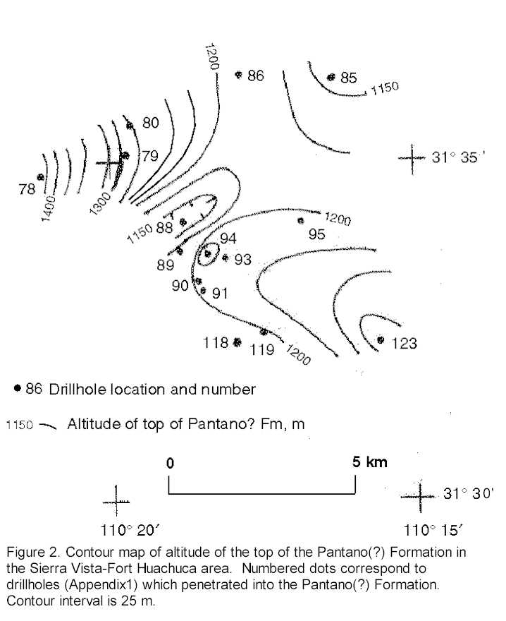
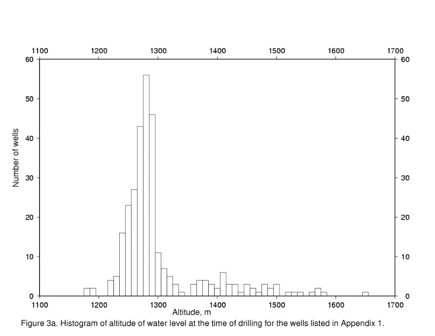
Table 2 summarizes some statistical properties of the altitudes of: the water table at the time of drilling; the top of the Pantano? Formation; and the top of bedrock as interpreted from the well logs. These altitudes are plotted as histograms in Figures 3a-3c. In Fig. 3a, the altitude of water table is a centrally peaked distribution with a tail towards higher elevations (1350-1600m). The wells in this tail are located on bedrock or shallowly covered bedrock in the Huachuca Mountains. Within the basin proper, the altitude of the water table is fairly well contained in the 50 m interval between 1240 and 1290m altitude even though the relief of the basin surface is over 300m. The basin behaves to a first approximation as an unconfined and permeable aquifer with the water level at about the same altitude throughout, like a bathtub of water.
Table
2. Statistical results for altitudes of water, top of Pantano? Formation,
and top of bedrock in the wells studied.
| Altitude in well of | Number of wells | Mini-mum, m | Maximum, m | Mean, m | Stand. Dev., m | Median, m | Mode, m | Note |
| Water | 301 | 1179 | 1653 | 1301 | 73.5 | 1280 | 1285 | 1 |
| Top of Pantano? Fm | 72 | 984 | 1570 | 1293 | 121.7 | 1303 | 1325 | 2 |
| Top of bedrock | 46 | 943 | 1577 | 1361 | 174.5 | 1404 | 1575 | 3 |
Notes:
1. Dry holes excluded.
2. Includes holes in exposed Pantano? Fm and excludes holes with zero thickness of Pantano? Fm between basin fill and bedrock.
3. Excludes holes starting in bedrock.Figure 3b shows the distribution of altitudes of the top contact of the Pantano? Formation in the wells studied. Note that this includes wells which began or "collared" in exposed Pantano? Formation and accounts for the peak in the distribution centered at 1400m. For the altitudes below the surface, the distribution is approximately normal with a mean of about 1275m and standard deviation of about 120 m and somewhat skewed toward higher elevations. The two peaked nature of the distribution may be due to the faulted nature of the western edge of the basin where most of the wells which encountered the contact are located.

Figure 3c shows a histogram of the distribution of the top contact of bedrock for the wells which penetrated into bedrock. Holes which were "collared" in bedrock are not included so that the distribution represents only holes in the basin reaching to bedrock. The distribution is multimodal and clearly skewed to higher altitudes because of the lack of deep holes. The multimodal distribution reflects the fact that the buried bedrock is a faulted topographic surface.

Gravity data were compiled from the gravity library of the Defense Mapping Agency and from data acquired for the mineral-resource assessment of the Coronado National Forest (Gettings, 1996). In addition, U.S. Geological Survey (USGS) personnel established 182 new stations for the current investigation. The resulting 1,521 data points were terrain corrected and the Complete Bouguer gravity anomaly value at each station was computed using standard USGS formulae as described in Gettings (1996). The resulting gravity anomaly map is shown in plate 3 and the gravity principal facts for the stations used are listed in Appendix 4. The Bouguer reduction density used in computation of the gravity anomalies was 2.67 g/cc (gram/cubic centimeter), and all observed gravity values are based on the observed gravity value of the gravity base station in the basement of the Gould-Simpson Building at the University of Arizona, Tucson. The data were compiled for digital use into grids of values at 0.5-km and 1.0-km intervals across the study area using minimum curvature as the interpolation technique (Briggs, 1974; Webring, 1991).
The gravity anomaly map (pl. 3) shows gravity anomaly relative maxima over the mountain ranges, the Tombstone Hills, and in an area of sparse bedrock exposures about 20 km northwest of Tombstone (pl. 1). Gravity station coverage is poorest in the Mule Mountains and consequently little is known of the detailed shape of the anomaly field in the Bisbee area. The Tombstone Hills and Whetstone Mountains areas are the only mountain areas with adequate gravity station coverage for regional geologic structural studies of the ranges themselves. The basin areas are generally marked by relative gravity anomaly minima or lows (pl.3). The areas of large gravity anomaly minima are much more restricted than the areas of alluvial basin fill on the geologic map (pl. 1), showing that the deep portions of the basin fill are restricted to subbasins within the valleys. The fact that the steep gravity anomaly gradients are well within the basin fill indicates that much of the basin areas are alluviated pediment surfaces eroded toward the mountains from the range-bounding faults. Gravity station coverage within the basin is good to excellent for the scale of the study (pl.3) except for the basin northeast of the Mule Mountains. This area appears to have a significant gravity anomaly minima associated with it and therefore a substantial depth of fill but is not considered further here due to lack of gravity station data.
The Tombstone subbasin is well defined by a northwest-trending gravity minima. The regional continuity and amplitude of the anomaly gradient along the southwest side strongly suggests a major fault as the boundary between the subbasin and the Tombstone Hills. Gettings and Gettings (1996) have modelled a gravity and ground magnetic profile across the Tombstone subbasin and continuing across the Tombstone Hills to Sierra Vista. Their results show that the subbasin may be as deep as 2 km beneath the profile track, but as much as 50% of the basin fill is probably Tertiary volcanic rocks, some of which are exposed in the area (pl. 1).
West of the Tombstone Hills, the gravity anomaly minima associated with the upper San Pedro basin (pl.3) has three local minima defining three subbasin areas separated by bedrock saddle points or highs. The largest anomaly minima, and therefore probably the area of largest depth of fill, is the Palominas subbasin, defined by a north-trending minima in the gravity anomaly field just west of Palominas (fig. 1). The Fort Huachuca-Sierra Vista area is an area of a bedrock high beneath the valley connecting the Tombstone Hills and the Huachuca Mountains in the subsurface. To the northwest, another anomaly minima defines the Huachuca City subbasin, which is also a north-trending gravity anomaly low with the largest minimum at the southern end, similar in form to the Palominas subbasin to the southeast. Finally, at Benson in the northern part of the map area (pl.3) there is a northwest trending anomaly minimum defining the subbasin there. It is notable that the San Pedro River location (pl.3) is completely uncorrelated with the deepest parts of the basin as defined by the gravity anomaly field.
Preliminary depth estimates for anomalies on the Bouguer gravity anomaly map (pl.3) were computed using an automated program which estimates the depth to source for gravity anomaly gradients which are sufficiently continuous to allow an estimate not overly affected by the noise level of the data. The method is based on estimation of the analytic signal of the potential field data from the horizontal gradient (Roest and Pilkington, 1993) and yields a depth to source, an estimate of the error of the depth estimate, and the trend of the gradient on which the estimate was made. By using the trends from all depth estimates regardless of error, one obtains a map of quantifiable trends in addition to the depth estimates. Usually, only the depth estimates with reasonably low error values are used for depth estimates. For this study, only depths with error estimates of 10% or less were used, although trends from all estimates were used to plot the trends. The method can be carried out on both gravity and magnetic field data. For gravity data, the method assumes the signal is coming from a thin horizontal layer and thus gives maximum depth estimates. For magnetic field data, the method corresponds to a thick source and the depth estimates are minimums. For this work, the gravity data were transformed to equivalent magnetic data using the pseudomagnetic transformation in program FFTFIL (Hildenbrand, 1983). Depths and trends were computed for both the gravity and pseudomagnetic datasets using a set of programs written by J. Phillips (written communication, 1998).
Figure 4a shows the results of these calculations for the gravity anomaly field, and figure 4b shows the results for the pseudomagnetic field. In both cases, the trend lines and depth estimate symbols are superimposed on the geologic map of pl. 1. The diameter of the depth estimate circle at map scale is the depth estimate at the center of the circle. Phillips (written communication, 1999) and other investigators have shown that the trend lines from the horizontal gradient method used here are sometimes displaced horizontally relative to the actual contact, due to the geometry of the real source not agreeing with the assumptions of the model. The displacement in the case of a fault is usually down dip. Study of figs. 4a and 4b in those places where the contact is known, shows displacements varying between 0 and 500 m, with approximately 200m being the most common. For the purposes of this study, these displacements are not important, but they should be borne in mind when using this work in any detailed study.
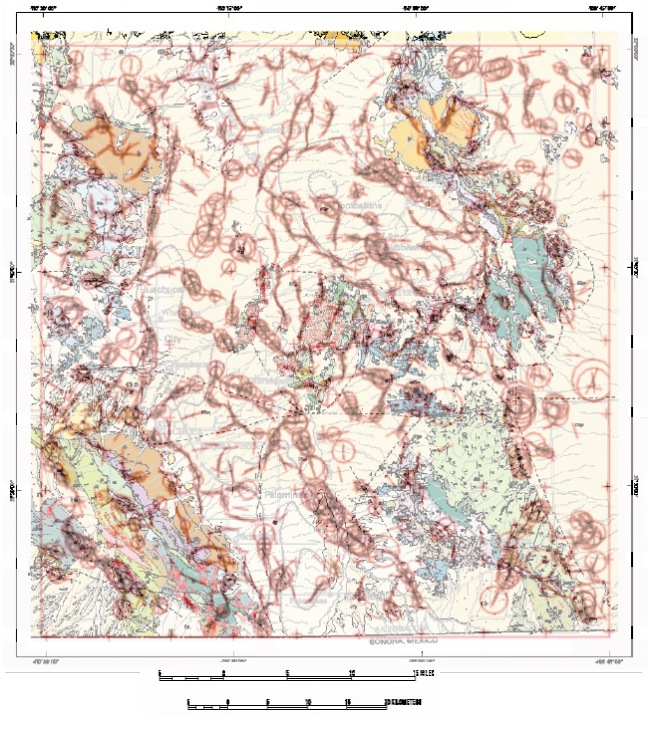
Figure 4a. Trends (line segments) and depth estimates
(diameter of circles at map scale) for sources of gravity anomalies computed
from the Bouguer gravity anomaly grid. Trends and depths are shown in red
superimposed on the geologic map of plate 1.
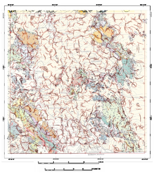
Figure 4b. Trends (line segments) and depth estimates
(diameter of circles at map scale) for sources of gravity anomalies computed
from the pseudomagnetic transformation of the Bouguer gravity anomaly grid.
Trends and depths are shown in red superimposed on the geologic map of
plate 1.
Fig. 4a shows a fairly continuous set of trends that mark the basin-bounding faults on the west side of the San Pedro basin and correspond well with known boundaries in the geologic data. Similarly, the bounding structures in the Tombstone subbasin are clearly identified, together with a number of quasi-linear features within the subbasin which appear to correlate with exposures of volcanic rocks (pl.1). Surprisingly, the Benson fault, which separates the Precambrian rocks from the Bisbee group rocks to the northeast at the northern end of the Whetstone mountains, has virtually no gravity anomaly expression. The trend analysis instead outlines a roughly circular structure beneath the Precambrian, Bisbee group, and fill to the north, and strongly suggests a buried intrusive "rafting" the northern Whetstone block structurally upward as suggested by Gettings (1996). The bounding trend for the subbasin in the Benson area appears to be a northwest extension of the trend defining the southwest edge of the Tombstone subbasin, rather than the Benson Fault farther south.
Trends in fig. 4b are much less continuous and more random in their directions. This is due mainly to the relative scarcity of (gravity) stations relative to the variability of the magnetic field. The pseudomagnetic transformation is essentially a differentiation operation and thus introduces noise into the computed grid, resulting in more dispersion in the trend directions. The lack of sufficient station density is a low pass filter on the gridded data; this results in many fewer areas from which reliable depth estimates can be computed. Nevertheless, the trends in fig. 4b do yield additional insight into the location of structural boundaries, and where depths are available, yield a depth estimate based on different assumptions. Ideally, the depths from fig4a and 4b should bracket the true depth to source where the sources are reasonably close to the model geometries. Many of the major structural boundaries are delineated on both figures 4a and 4b. In particular, the west-southwest trending boundaries in the Sierra Vista-Fort Huachuca are well defined. At least some of these boundaries appear to be faults of shallow horsts and grabens of the bedrock high between the Huachuca City and Palominas subbasins. Bedrock of one or more of these horsts has been sampled by drillholes listed in Appendix 1.
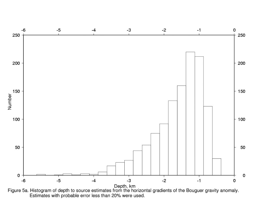
Histograms of the computed depth estimates with error estimates of less than 20% are plotted in figures 5a and 5b. Fig. 5a shows the distribution of depths for estimates computed from the Bouguer gravity anomaly field, and fig 5b shows those calculated from the pseudomagnetic transformation of the gravity anomaly. Table 3 lists the summary statistics for these estimates and from figs 5a and 5b and Table 3 it is obvious that the pseudomagnetic transformation estimates are less than those from the gravity anomaly itself, but the distribution shape is essentially unchanged. It should be noted that the deeper depths (especially deeper than 2 km) may be due to density changes within the bedrock rather than the basin fill-bedrock interface. The most frequent depths in the distributions are in the 1.0-1.25 km range suggesting that the largest areas of the subbasins are about this depth. The shallowest depths are about 0.4 km and correspond mainly to depths to the tops of the range-bounding faults beneath basin fill, that is, the edge of the buried pediment surface. In general, areas of exposed bedrock have too small a station density to yield shallower depth estimates even though the gradient corresponds to a contact on the surface. The close coincidence of the depth estimate location and contact implies that the contacts are steeply dipping. The deeper depth estimate in these cases is due to the low pass filtering effect of the grid generation process plus the lack of closely spaced station data.
_________________________________________________________________________
Table
3. Summary statistics for computed depths to source from the Bouguer gravity
anomaly dataset.
| Depths estimated on: | Number of points | Minimum, km | Maximum, km | Mean, km | Stand. Dev., km | Median, km | Mode, km |
| Bouguer gravity
anomaly |
1227 | 0.389 | 5.438 | 1.603 | 0.751 | 1.410 | 1.125 |
| Pseudo-magnetic transform | 558 | 0.387 | 3.736 | 1.151 | 0.484 | 1.050 | 0.875 |
Estimation of basin geometry from the geologic and geophysical data
The procedure used to model the shape of the basin and the thickness of the basin fill units from the geologic and geophysical data is a refinement of that used by Gettings and Houser (1997) and is comprised of a number of steps described in detail below. The main steps are as follows.
1) Define the density contrast versus depth functions to be used for the basin fill and the Pantano? Formation from density measurements and well logs.
2) Estimate the gravity anomaly field due to the bedrock using gravity stations located on bedrock, modified gravity anomalies at wells which penetrated into bedrock, and from appropriately upward continued estimates of bedrock gravity anomalies over the basin.
3) Calculate the gravity anomaly field due to the basin by subtraction of the bedrock gravity anomaly from the observed complete Bouguer gravity anomaly.
4) For wells which penetrated into the Pantano? Formation, calculate the depth to bedrock from the residual gravity anomaly and the known thickness of basin fill.
5) Calculate a grid of depth to bedrock (base of the Pantano? Formation) values from the residual gravity anomaly, controlled by the location of bedrock in outcrop and in wells (those that penetrated to bedrock and those that penetrated into Pantano? Formation described in step 4) and using a preliminary grid of thickness of basin fill from outcrop and well control.
6) Calculate a grid of thickness of basin fill using the depth to bedrock grid of step 5, the residual gravity anomaly grid, and all control points from outcrop and wells.
7) If the model does not fit the gravity anomaly field sufficiently well, repeat steps 5 and 6; if there is still poor agreement, steps 2 to 6 must be repeated with additional data or model assumptions to provide further constraints.In this study, step 7 was not needed because the final model anomaly fit the basin anomaly to within the limits of definition due to the uncertainty in the bedrock gravity anomaly. However, steps 1-6 were performed numerous times because of newly discovered well data and due to the correction of errors discovered in the various datasets.
An element critical to successful estimation of depths from gravity anomaly data is knowledge of the density of the material filling the basin and the density of the bedrock below. Density data from well logs within the upper San Pedro basin are available for seven test wells on the Fort Huachuca Military Reservation (United States Army, 1972, 1974) and for two deep petroleum exploration wells (Schlumberger geophysical logs done in 1981 and 1982, available at the Arizona Geological Survey, Tucson). Figure 6 shows the measured densities as a function of depth for Test Well 8 (well 85, appendix 1) and interval averages for the deep petroleum exploration well drilled in 1982 by Phillips Petroleum Company (#A-1) located about 4 km east of Whetstone, (table 1; well 30, appendix 1). Note that the upper 324 m (1,062 ft) of the Phillips well were not logged for density.
All densities were determined by a downhole compensated gamma-gamma formation density logging tool. Although the data show large variability, they generally show increasing density with depth and changes of density with lithology. The section of the log of Test Well 8 (fig. 6) from 11 to 193 m corresponds to density in the basin fill sediments both above and below water table, which stood at 75 m (245 ft) at the time of logging. The interval from 193 to 395 m corresponds to the density of the consolidated sediments that are interpreted to be the Pantano? Formation. The density variations over short vertical distances in the log of Test Well 8 are interpreted to be due to changes in the proportion of silt, sand, and gravel, as well as degree of cementation. The approximately linear increase in density with depth of the basin-fill unit is interpreted to be due mainly to compaction of the unconsolidated basin fill. It is notable that there is not an obvious increase in density at the water table (75 m); this can only mean that the porosity is low and may indicate that there is not a large proportion of connected pore space in this interval of the material penetrated by Test Well 8.
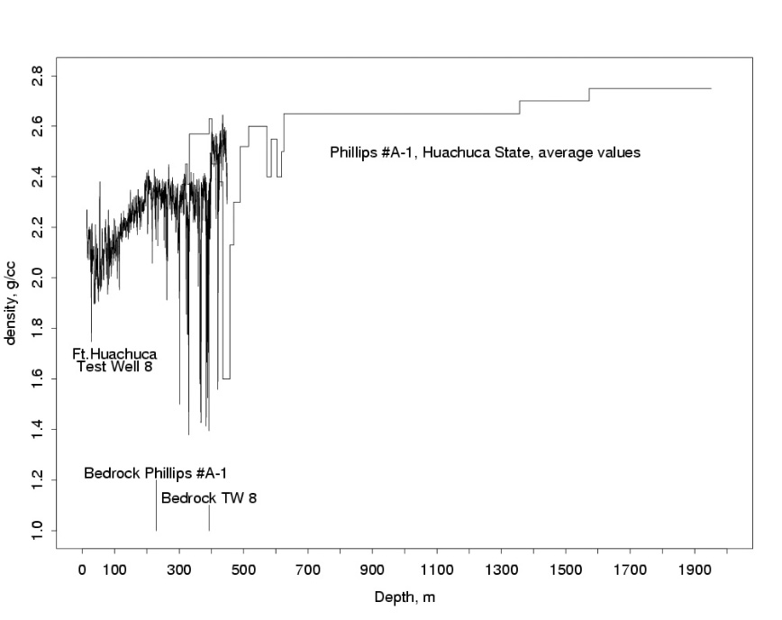
Figure 6. Compensated gamma-gamma formation density logs of two drillholes which penetrated to bedrock. Values shown for the Phillips #A-1 hole are interval averages.
Also shown in figure 6 are interval average densities for the density log of Phillips Petroleum A-1, Huachuca State well, determined by averaging more or less constant density segments of the log by eye, as the log has not yet been digitized. All of the log is in bedrock of the Cretaceous and Jurassic Bisbee Group and older formations (Table 1) and serves as a good example of how variable the bedrock density function may be. The thickness-weighted average bedrock density of the log for the interval shown on figure 6 is 2.65 g/cc, which is taken as the average bedrock density for the area in this study. This value corresponds closely with the Bouguer density of 2.67 g/cc used in the reduction of the gravity data.
Density functions which are a function of depth present analytical difficulties in gravity anomaly model calculations, so the segment of figure 6 that shows increasing density with depth of basin fill is approximated with three constant mean values for intervals as tabulated in table 4. The density contrast, that is, the difference between the sediment and the bedrock density, is shown in figure 7. Note that more intervals are used in the shallow part of the function where the density changes with depth are large. The shallow layers also have a larger effect because the gravitational force varies as the inverse square of distance, so it is important to model them adequately. An 11 m thick uppermost layer corresponding to dry, unconsolidated surficial alluvium has been included in the density contrast function.
Table
4. Density versus depth functions for the basin fill, Pantano? Formation,
and bedrock. Density contrast is sediment
density minus bedrock density.
| Unit | Depth (ft) | Depth (m) | Density
(g/cc) |
Density
contrast (g/cc) |
| basin fill | ||||
| dry | 0-36 | 0-11 | 1.85 | -0.80 |
| dry/saturated | 36-381 | 11-116 | 2.10 | -0.55 |
| saturated | 381-499 | 116-152 | 2.20 | -0.45 |
| saturated | 499-633 | 152-193 | 2. 27 | -0.38 |
| saturated | 633- | 193- | 2.27 | -0.38 |
| Pantano? Formation | ||||
| saturated | 0-1312 | 0-400 | 2.35 | -0.30 |
| saturated | 1312- | 400- | 2.35 | -0.30 |
| Bedrock (average) | 2.65 | 0.00 |

Figure 7. Density contrast function relative to bedrock adopted for this study.
Separation of the basin gravity anomaly
The interpretation of gravity anomaly data depends on the separation of the anomaly due to the geologic bodies of interest from the observed anomaly, which is the total gravity anomaly from all sources. Numerous methods are available for this procedure, but most are numerical methods that may or may not be geologically reasonable. The method used here follows that of Saltus and Jachens (1995), and is regarded as the best for this study because it defines the regional field using the gravity anomaly field from the bedrock of the surrounding ranges and from wells within the basin which intersected bedrock. Before discussing the details of the regional anomaly field estimation, a digression to describe the model used to calculate the gravity effect of a basin from its fill thickness, or to calculate the depth of fill from the basin gravity anomaly is necessary. The model was used repeatedly in this work to calculate gravity effects or thicknesses.
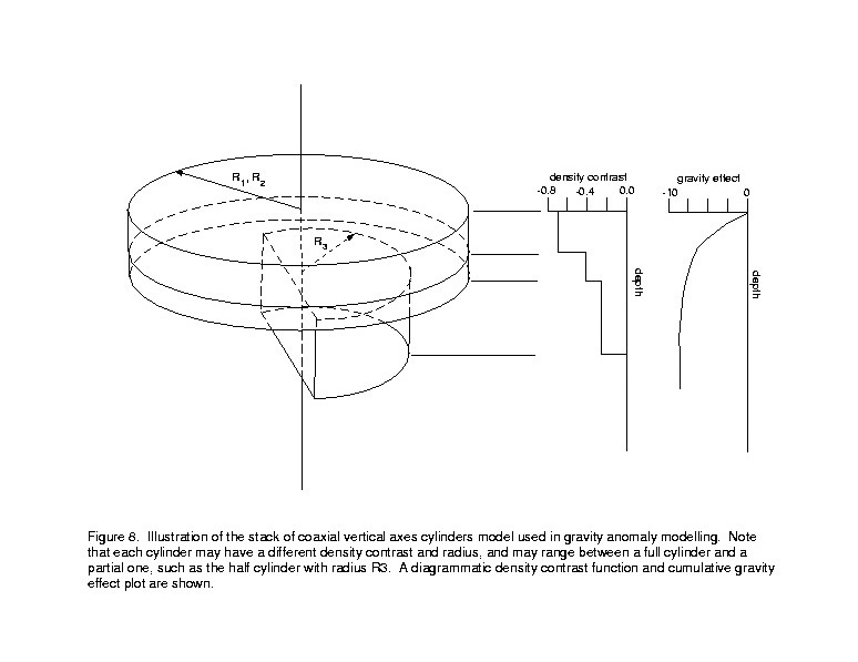
Using the density contrast functions discussed above, depths to bedrock can be estimated from the gravity anomaly. Depths are traditionally computed using an infinite horizontal slab model for the various density layers because of computational simplicity (for example, see Litinsky, 1989). However, the infinite slab formula is independent of depth to the slab and has infinite mass, leading to depth estimates that are too shallow. With the ready availability of computers, finite models are easily used to produce more realistic estimates. For this work, the finite right circular cylinder with vertical axis was used. For points on the axis, the exact solution is available (Duska, 1958). The model then consists of a stack of cylinders with coincident axes, each with a density contrast and thickness corresponding to the density contrast function of figure 7 and a radius appropriate for the basin being modeled (figure 8). When a site is located near a gravity anomaly gradient interpreted to be a fault, partial cylinders may be used as shown in the lower cylinder of fig. 8. This feature allows the interpreter to get accurate depths in the footwall right up to the fault, and the overlying cylinders model the fill on the pediment surface quite accurately. The partial cylinder gravity effect is obtained by calculating the effect of the missing part of the cylinder approximately using a series of partial cylindrical annuli and subtracting this effect from that for a whole cylinder.
Computer programs were written for several versions of this model, all of which use the density contrast functions for the basin fill and the Pantano? Formation described above. For the estimation of gravity effects, a version was written which uses the depth to Pantano? Formation and bedrock as input. Another version uses the depth to Pantano? Formation and residual gravity anomaly to calculate depth to bedrock using the method of bisection. Both of these programs additionally require radii and fraction of the cylinders as input parameters. Finally, there are two programs written to work on grids of residual gravity anomaly data, using grids of depth constraints. One of these programs uses a grid of depth to the Pantano? Formation and a grid of drillhole and outcrop depths to bedrock to calculate the depth to bedrock for all grid points in the basin. The other program uses a grid of depth to bedrock and a grid of drillhole and outcrop depths to the Pantano? Formation to calculate the depth to the Pantano? Formation for all grid points in the basin. These two programs use the stack of cylinders model for the grid point being calculated and a stack of finite (vertical) lines of mass for grid points off axis but still in the basin. No fractional cylinders are used and needed radii and distances are defined by the grid. Listings of the code for these four computer programs are given in Appendix 5.
For this work the upper basin fill or the Pantano? Formation functions were used as required by the log of the well. Because the density logs do not show much sensitivity to the presence of water, the values were not adjusted for the depth to water table.
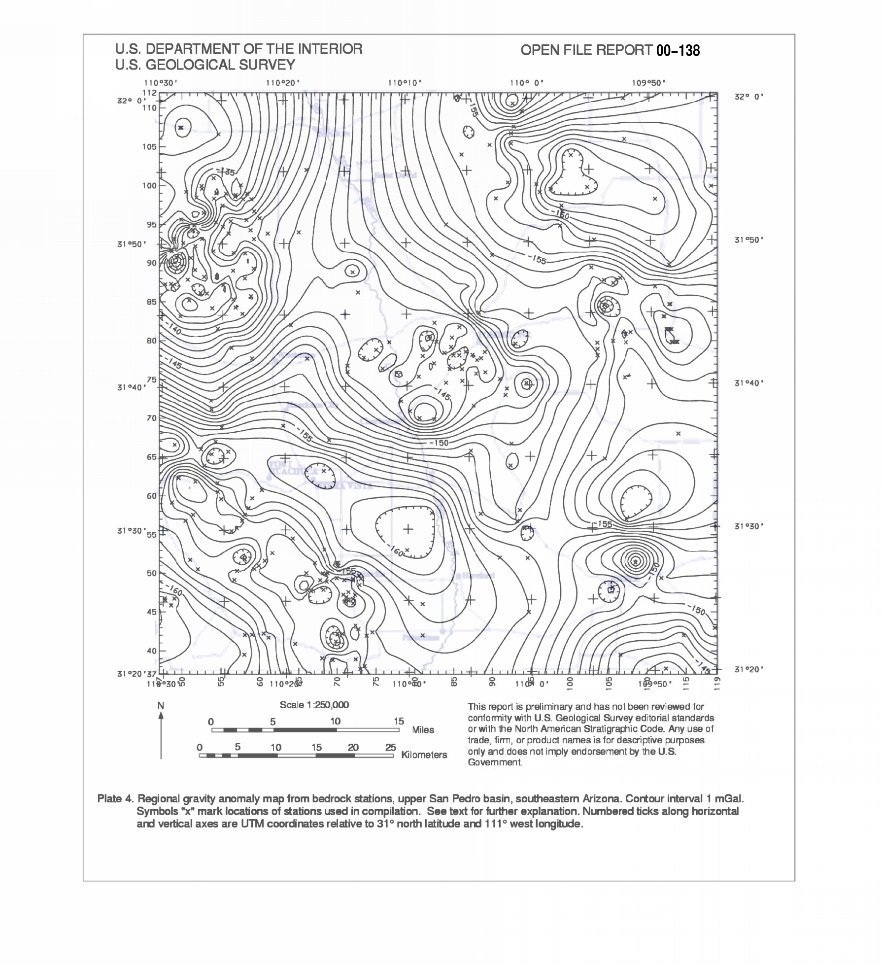
Based on the assumption that the rocks exposed in the adjacent ranges are likely to be the same as those that underlie the upper San Pedro basin, the regional field was defined by generating a coarse interval grid (5-km in this case) of Complete Bouguer gravity anomaly values from stations that are not located on upper basin fill or on Pantano? Formation. At each of the wells that penetrated into bedrock, the gravity effect of the basin fill and Pantano? Formation was calculated using the density contrast functions and software described above. This computed value was then added to the Complete Bouguer gravity anomaly value at each well location to yield the value that would be observed if the basin sediments were not present (Appendix 2). For this study, 206 stations were located on bedrock. These stations, together with the calculated values at 42 well locations that penetrated to bedrock (App. 2) and 10 locations on bedrock interpolated from the Complete Bouguer gravity anomaly map (pl. 3) where there were no station data, were used to calculate the coarse interval grid. Grid values for grids in this report were calculated by the method of minimum curvature (Briggs, 1974). This method of calculation will generate steep gradients at the edges of areas with no data points, so a coarse grid interval is used in a first pass to obtain a smooth interpolation. The grid is then recomputed using both the data for the coarse grid and the coarse grid points themselves to obtain a smooth grid at the same interval as the complete Bouguer gravity anomaly grid.
One additional complication arises in this process in parts of the basin where there are no drillholes to bedrock and thus no regional gravity control points. In these areas, the value of regional gravity estimated by the minimum curvature grid generation process is the value expected if the bedrock were in outcrop at the surface, since it is being interpolated from areas of bedrock outcrop. In fact, the bedrock in the basin is buried by the basin fill and thus the gridded values should be upward continued by a distance equal to the depth of burial. Since the depth of the basin is an unknown, one cannot calculate the continuation directly. Instead, "phony" stations are introduced where needed using a simplified continuation procedure discussed below. The "phony" stations are calculated by continuing the values from the coarse grid at points where control is needed due to lack of drillhole control. For this study thirteen "phony" stations were used. Two of these were in the Palominas subbasin; the others were in areas of poor gravity station coverage over basins such as south and west of Benson, east of Tombstone and Bisbee, and northeast of the Dragoon Mountains. These stations are included on plate 4 and can be identified as those which do not correspond to a drillhole to bedrock (pl. 2) and do not occur on bedrock outcrop (pl. 1). For purposes of the continuation procedure, a rough depth estimate from the estimated basin anomaly from the complete Bouguer gravity anomaly (pl. 3) using the stack of cylinders model was used.
In order to calculate a simple upward continuation factor, the continuation integral for a simple "plateau" anomaly was calculated. This corresponds to a mean anomaly due to bedrock of a range of the order of 20 km characteristic size. The upward continuation integral is (Grant and West, 1965)

where
![]()
is the data surface.
Take the observation point ![]() to
be (0,0,z) where
to
be (0,0,z) where ![]() , then
, then ![]() .
Now suppose that the gravity anomaly
.
Now suppose that the gravity anomaly ![]() is
a constant (boxcar function) within the rectangular area and zero elsewhere
is
a constant (boxcar function) within the rectangular area and zero elsewhere
![]()
![]() otherwise.
otherwise.
Although this function is not strictly a potential
field function because of the discontinuities at ![]() and
and ![]() ,
we are not concerned about the details of anomaly shape at the boundaries
since upward continuation at the center of the rectangle is the goal. One
can assume the actual anomaly shape change occurs continuously between
grid points. Integration yields
,
we are not concerned about the details of anomaly shape at the boundaries
since upward continuation at the center of the rectangle is the goal. One
can assume the actual anomaly shape change occurs continuously between
grid points. Integration yields
as the desired relation.
To evaluate the accuracy of this formula for real cases, two tests were carried out. In the first, the gravity effect of a unit density sphere of radius 5 km with center at 10 km depth was evaluated. The upward continued field over the sphere was evaluated at 1 km and 5 km upward continuation distances. The upward continued field was also evaluated by Fourier transform techniques (program FFTFIL, Hildenbrand, 1983) and the above formula. For 1 km continuation distance, FFTFIL gave a value 0.75% too large while the formula above gave a value 0.50% too small compared to the exact solution. For 5 km distance, compared to the exact results, FFTFIL was 6.8% too large and the formula 25% too small, a result to be expected since at this distance the source is much more a point source than a "plateau" anomaly. In the second test, a grid was computed with gravity anomaly values equal to zero except in a rectangle 20 km by 30 km in the middle, where they were set to 10 mGal. Both FFTFIL and the formula were evaluated for upward continuation distances of 1, 2, and 3 km. For 1 and 2 km distances, the formula was about 3% smaller than FFTFIL, and for 3 km continuation, it was about 6% smaller than FFTFIL. From the sphere comparison, we conclude that FFTFIL overestimates the value whereas the formula underestimates them and thus the errors in the second test must partially cancel. For the application here, an error of 3% or less is acceptable as the determination of the bedrock regional anomalies are probably less certain than 3% in any case. Here we are only interested in how to reduce the value for bedrock due to burial beneath the basin. Dimensions of 20 km by 20 km and continuation depths of 0-2 km (about 10% or less of the horizontal extent of the source) are the appropriate values so that the simple approximation of the formula above is entirely adequate.
The coarse grid (5 km interval) was recomputed using the upward continued "phony" stations in addition to the original points, and then recomputed at 1-km intervals as described above to yield the regional gravity anomaly field shown in plate 4. This grid was then subtracted from the complete Bouguer gravity anomaly grid generated using all stations to yield a residual gravity anomaly grid shown as a contour map in plate 5. Because the density-depth functions are fixed in the formulation of Saltus and Jachens (1995), whereas here the object is to find the variations in the depth to the intra-sedimentary contact, the modeling scheme is carried out somewhat differently from that described by those authors. In this study, the residual gravity anomaly, shown in plate 5, forms the basic data for analysis.
Estimation of depth to bedrock
Using the residual gravity anomaly defined above, depths to bedrock were computed at all wells that penetrated into the Pantano? Formation but not to bedrock. For each of these wells, parameters defining the average radii and fractions of cylinders to be used were defined by overlaying the well locations (pl.2), residual gravity anomaly (pl.3) and geologic map (pl.1). The stack of cylinders model was then used to compute depth to bedrock. Appendix 3 summarizes the parameters and the final estimated depth to bedrock for the 56 wells that penetrated into the Pantano? Formation.
Next, a grid of bedrock depth estimates at a 1-km interval was computed using the following three grids as controls. (1) A grid was constructed that contained the outline of bedrock outcrop and that flagged all grid cells on bedrock as zero depth. Into this grid were inserted the locations and control depth points from the 42 wells of Appendix 2 and the 56 wells of Appendix 3. (2) A second grid was constructed by minimum curvature interpolation using the bedrock outcrop and the depths to the top of the Pantano? Formation from the wells of appendices 2 and 3 as data points. This grid is the first estimate of the thickness of basin fill. (3) The residual gravity anomaly grid of plate 5 was used to compute depth estimates using the stack-of-cylinders model and using the second grid for the depth to the Pantano? Formation and the first grid for control points. The depth-to-bedrock grid is shown in plate 6 at a contour interval of 0.1 km.
Estimation of thickness of basin fill
Depth to the contact between the basin fill and the Pantano? Formation was computed from the the residual gravity anomaly (pl. 5), the estimated depth to bedrock (pl. 6), and the density contrast-depth functions of figure 7 using the following algorithm. First, the density contrast-depth function (table 4) was split into one function for the upper basin fill, and a second function for the Pantano? Formation. For a given total depth (depth to bedrock), one can compute the gravity anomaly as a function of the depth to the contact between the upper basin fill and the Pantano? Formation. Then for the residual basin anomaly at that point, one can interpolate the depth to the contact from the gravity anomaly-depth function just computed. This proceeds for all points in the grid. Points on bedrock are not computed, and points where depths to bedrock or Pantano? Formation are known (for example, wells in appendix 2) are not allowed to change. The model gravity effect from the new model is then computed and compared to the residual gravity anomaly grid. Differences between the model and the gravity anomaly data are then used to assess the quality of the gravity model.
Thus, this procedure finds the depth to Pantano? Formation that best fits both the gravity anomaly and the estimated depth-to-bedrock datasets, constrained by the known depths to the Pantano? Formation. It must be noted that because of the inherent ambiguity of solutions to the gravity anomaly field, iteration has to be used with caution, and the process is more one of interpolation of the known depths using the gravity anomaly as a guide, rather than an iterative procedure. If necessary, the depth to bedrock can then be adjusted and the procedure repeated. For this study, the rms misfit between the model and the residual gravity anomaly (pl.5) was 0.65 mgal, and further adjustment is not justified as the uncertainty in the residual gravity anomaly value is at least as large. In the course of carrying out these computations, it was found to be necessary to assume the depth of fill in the area of wells 99, 104, and 106 because the algorithm yielded small thicknesses of basin fill relative to the thickness of Pantano? Formation in this area. We could find no geologic justification for this being the case. We therefore assumed that the depth to the top of Pantano? Formation was about the same as to the south at well 108 and to the northwest at 105, for example, and used a depth of 200 m for the top of Pantano? Formation at wells 99, 104, and 106. The deepest well in this cluster, 104 (app. 1), penetrated only basin fill in the total depth of 183 m.
Plate 7 shows the depth to Pantano? Formation computed using the residual gravity anomaly grid (pl. 5), the depth to bedrock grid (pl. 6) and the control grid described above. Plate 7 shows that areas where the basin fill is thicker than 200 m form a belt in the basin about midway between bedrock outcrop on the west and the San Pedro River on the east. Basin fill is thicker over the two subbasins; the larger subbasin extends from the area of Huachuca City north to Whetstone (pl.1), and the other is southwest of Hereford (pl.1). The depth of basin fill in the bedrock high area between the two subbasins is generally 200 m or less (pl. 7).
In general the agreement of calculated depths for the grid with control values is good. Some areas have several control points within a one-km grid cell and the editing process assigns a value to the grid point equal to the last one in the list falling in that cell. This is not a serious difficulty because from field observations we know that the variations in the degree of consolidation of the Pantano? Formation and the possibility of relief on the contact of at least 20 m mean that we can only estimate an average depth in any case. Real variations in the physical properties of the basin units probably preclude any more accurate knowledge of the interface over small areas.
Based on reasonable approximations, we have constructed a basin-fill model that satisfies constraints from geologic, well log, and gravity anomaly data. This model indicates that within the study area, the upper San Pedro basin is composed of a series of structurally controlled subbasins with intervening bedrock highs. Some of the highs outcrop, such as the Tombstone Hills, while others are buried beneath the alluvial fill of the basin. The subbasins are approximately 1.0 to 1.7 km in depth, and generally filled with a consolidated alluvial unit overlain by an unconsolidated basin fill unit. The only areas of significantly thick basin fill are within those areas which have already been established by well logs. North of Huachuca City, the consolidated basin unit, the Pantano? Formation, is not present at least locally in wells and does not outcrop.
We have included an animation of a rendering of the depth to bedrock and depth to the top of the Pantano(?) Formation. In the animation, the grid of computed bedrock depths (pl. 6) is the smooth colored surface and the colored wire frame is the depth to the top of the Pantano(?) Formation (pl. 7). The depth estimates from the gravity anomaly and pseudomagnetic transformation of the gravity anomaly (figs. 4a and 4b) are also shown. The animation shows the surfaces from above and below and multiple viewpoints in order to help visualize the subbasins and the bedrock highs. Although a few of the depth estimates are above the model surface, most ar well below it and represent maximum depth estimates.
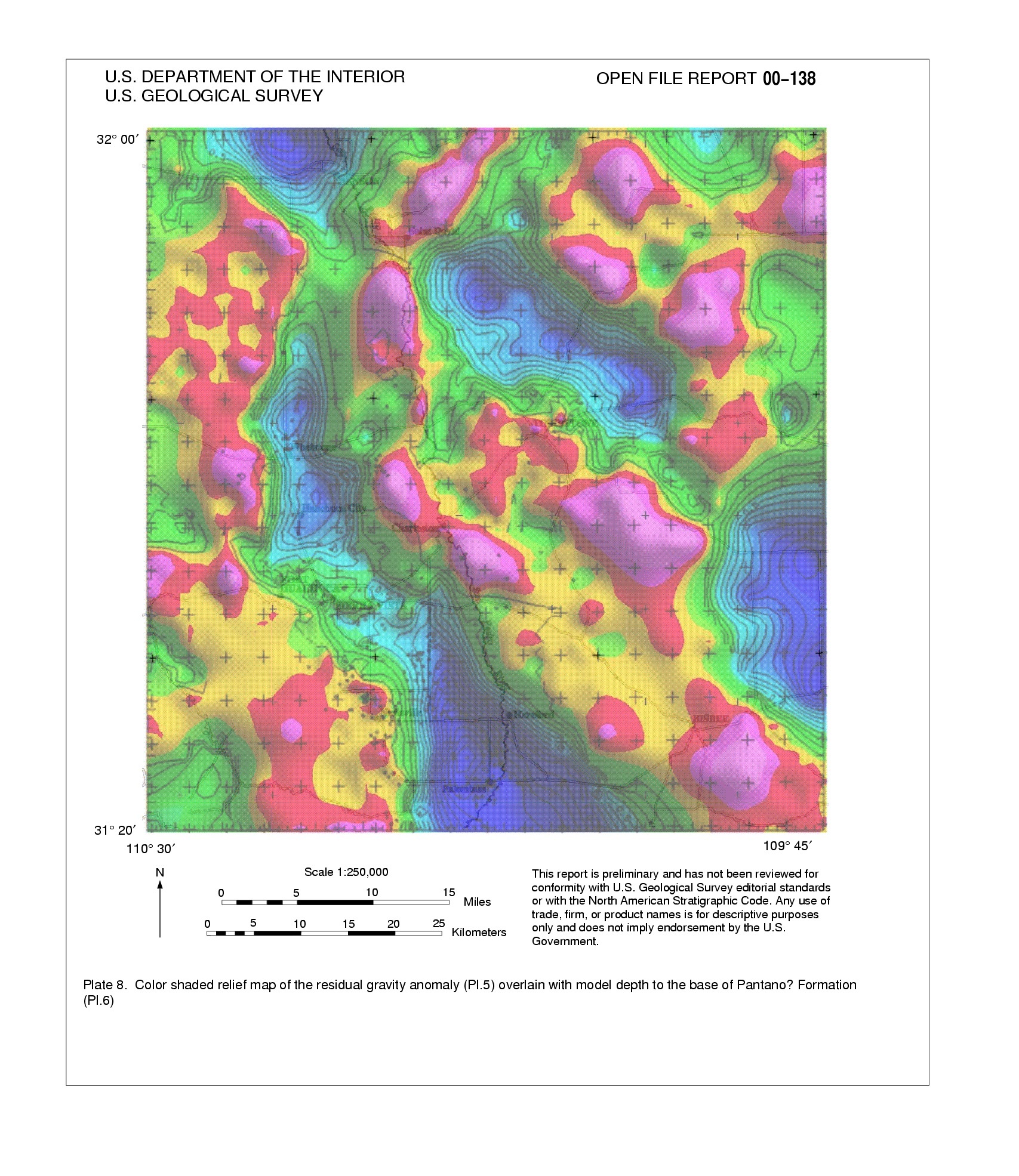
Plate 8 shows a color shaded relief image of the residual gravity anomaly pl. 5) with the contours of the calculated depth to bedrock (pl.6) superimposed. Areas of pl. 8 where contours are lacking correspond to areas of shallow cover or outcrop (note that the first contour is the 0.1 km depth contour to keep the figure uncluttered). Examination of areas of bedrock outcrop in pl.8 (see pl. 1 for geologic map) shows that there are significant gravity anomalies within the bedrock areas. We expect that the same kind of relief of the gravity anomaly field is present in the bedrock beneath the basin fill although the amplitudes of the anomalies will be less because of the upward continuation effect from burial beneath the basin fill. In this study, we have attributed all negative gravity anomalies in the basin area to the thickness of less dense alluvial units. However, some of the negative anomalies over the basin may in fact be due, at least in part, to low density units in the bedrock. If this is the case, then the modelled basin depths will be too deep. Therefore the model depths of this study should be viewed as maximum depths of fill. The opposite case, namely where a positive bedrock anomaly masks part of the basin fill anomaly does occur between Sierra Vista and Charleston, but we believe it has been adequately accounted for by the control from wells and analysis of the aeromagnetic data (Gettings, 1999). In any case this effect of positive anomalies is not as serious a limitation because there are not many rocks in the bedrock more dense than the average density of 2.67 g cm-3 used in the model. Large areas of mafic intrusive rocks which might be significantly more dense are not present in outcrops within the study area (pl.1).
We have identified a number of previously unrecognized faults and several outcrops of bedrock (pl. 1). The shape of the subbasins is predominantly controlled by the pattern of faulting. Some of the faults may affect the course of the river. The possibility that these and other faults may also control the movement of ground water should be investigated. In all of the subbasins defined in this study, the subbasin shape appears to be controlled by a combination of northwest-southeast trending older structures and younger approximately north-south trending structures. The older trend expresses the northeast-southwest directed extensional tectonic event, and the younger the more recent east-west directed Basin and Range extensional event.
We gratefully acknowledge the many people who assisted in collecting geologic and geophysical data for this project. Karen Baird established 66 new gravity stations in the study area. Don Pool contributed data for 46 gravity stations in critical parts of the eastern Fort Huachuca area. Frederick Houser assisted in the geologic mapping. The Arizona Geological Survey gave permission to study well cuttings. Funding for this project was provided in part by the United States Army, Fort Huachuca Garrison.
Balcer, R.A., 1984, Stratigraphy and depositional history of the Pantano Formation (Oligocene-early Miocene), Pima County, Arizona: Tucson, University of Arizona M.S. thesis, 107 p.
Briggs, I.C., 1974, Machine contouring using minimum curvature: Geophysics, v.39, p. 39-48.
Brown, S.G., Davidson, E.S., Kister, L.R., and Thomsen, B.W., 1966, Water Resources of Fort Huachuca Military Reservation, southeastern Arizona: U.S. Geological Survey Water-Supply Paper 1819-D, 57p.
Demsey, K.A., and Pearthree, P.A., 1994, Surficial and environmental geology of the Sierra Vista area, Cochise County, Arizona: Arizona Geological Survey Open-File Report 94-6, 14p., scale 1:24,000.
Dickinson, W.R., 1991, Tectonic setting of faulted Tertiary strata associated with the Catalina core complex in southern Arizona: Geological Society of America Special Paper 264, 106 p.
Drewes, Harald, 1980, Tectonic map of southeast Arizona: U.S. Geological Survey Miscellaneous Investigations Series Map I-1109, scale 1:125,000.
Drewes, Harald, 1996, Geologic maps of the Coronado National Forest, southeast Arizona and southwest New Mexico: U.S. Geological Survey Bulletin 2083-B, pp. 17-41, pls 2-4.
Duska, L., 1958, Maximum gravity effect of certain solids of revolution: Geophysics, v. 23, p. 506-519.
Gettings, M.E., 1996, Aeromagnetic, radiometric, and gravity data for Coronado National Forest, in du Bray, E.A., ed., Mineral resource potential and geology of Coronado National Forest, Southeastern Arizona and Southwestern New Mexico, U.S. Geological Survey Bulletin 2083-D, p. 70-101.
Gettings, P.E, and Gettings, M.E.,1996, Modelling of a magnetic and gravity anomaly profile from the Dragoon Mountains to Sierra Vista, southeastern Arizona: U.S. Geological Survey Open-File Report 96-288, 15p.
Gettings, M.E., and Houser, B.B., 1995, Preliminary results of modeling the gravity anomaly field in the upper San Pedro basin, southeastern Arizona: U.S. Geological Survey Open-File Report 95-76, 9p.
Gettings, M.E., and Houser, B.B., 1997, Basin Geology of the upper Santa Cruz Valley, Pima and Santa Cruz counties, southeastern Arizona: U.S. Geological Survey Open-File Report 97-676, 40p.
Grant, F.S., and West, G.F., 1965, Interpretation Theory in Applied Geophysics, McGraw-Hill Book Company, New York, 584 pp.
Hildenbrand, T.G., 1983, FFTFIL: A filtering program based on two dimensional Fourier analysis: U.S. Geological Survey Open-File Report 83-237, 31 p.
Houser, B.B., Richter, D.H., and Shafiqullah, M., 1985, Geologic map of the Safford quadrangle, Graham County, Arizona: U.S. Geological Survey, Miscellaneous Investigations Series Map I-1617, scale 1:48,000.
Litinsky, V.A., 1989, Concept of effective density -- key to gravity depth determinations for sedimentary basins: Geophysics, v. 54, p. 1474-1482.
Moore, R.B., 1993, Geologic map of the Tombstone volcanic center, Cochise County, Arizona: U.S. Geological Survey Miscellaneous Investigations Series Map I-2420, scale 1:50,000.
Roest,W.R., and Pilkington, M., 1993, Identifying remanent magnetization effects in magnetic data: Geophysics, v. 58, p. 653-659.
Saltus, R.W., and Jachens, R.C., 1995, Gravity and basin-depth maps of the Basin and Range Province, Western United States: U.S. Geological Survey Geophysical Investigations Map GP-1012, scale 1:2,500,000.
Webring, M.W., 1991, Minimum curvature gridding of scattered data: U.S. Geological Survey Open-File Report 91-1224.