
![]()
High Resolution, Low Altitude
Aeromagnetic
and Electromagnetic Survey of
Mt Rainier
By
V. L. Rystrom, Carol A. Finn and Maryla Deszcz-Pan
Open-File-Report 00-027
![]()
In October 1996, the USGS conducted a high resolution airborne magnetic and electromagnetic survey in order to discern through-going sections of exposed altered rocks and those obscured beneath snow, vegetation and surficial unaltered rocks. Hydrothermally altered rocks weaken volcanic edifices, creating the potential for catastrophic sector collapses and ensuing formation of destructive volcanic debris flows. This data once compiled and interpreted, will be used to examine the geophysical properties of the Mt. Rainier volcano, and help assist the USGS in its Volcanic Hazards Program and at its Cascades Volcano Observatory .
Aeromagnetic and electromagnetic data
provide a means for seeing through surficial layers and have been tools
for delineating structures within volcanoes. However, previously acquired
geophysical data were not useful for small-scale geologic mapping. In this
report, we present the new aeromagnetic and electromagnetic data, compare
results from previously obtained, low-resolution aeromagnetic data with
new data collected at a low-altitude and closely spaced flightlines, and
provide information on potential problems with using high-resolution data.
![]()
PAGE OUTLINE
Short History of Aeromagnetic Surveys
Next Generation Aeromagnetic Surveys
Electromagnetic Resistivity Survey
Download Data Files
![]()
Prior to the use of GPS navigation, surveys were located by matching photographs and film taken from a moving aircraft with topographic maps. Elevation was recorded by barometers which converted pressure to elevation. The typical survey was flown at a constant barometric elevation. An old (1981) survey of Mt. Rainier (Open File Report: OF 82-0547) was flown with a line spacing of 1.6 miles (1 km) at a constant barometric elevation of 16,500 ft (~5500 m). This terrain clearance for this survey varied from about 2000 ft (~670 m) over the summit to 12,500 ft (~4150 m) above the flanks of the volcano. Magnetic data collected from the magnetometers were recorded at 1 sample per second which resulted in approximately one data point per 150-200 feet (50-70 meters) on the ground. The data was then mapped in contour form.
Elevation approximately 16,500 ft, flown at a level flight path.
Line spacing approximately 1 km apart.
Resulting images from 1981 Mt. Rainier flight:
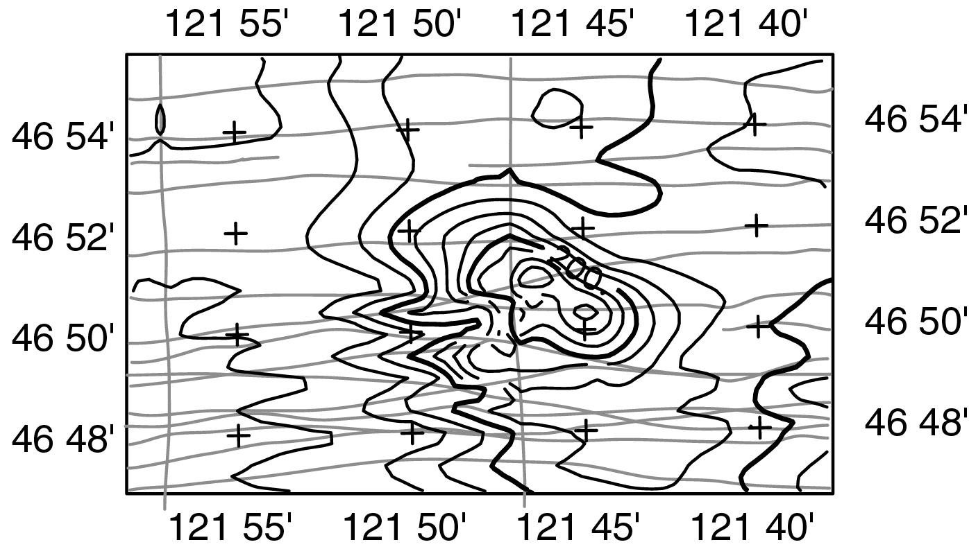
Magnetic data represented in contour form.
Before the late 1980's contour mapping was the standard representation of magnetic data. The flight lines (horizontal lines and two tie lines) show the path flown by the airplane. The "herringbone" appearance of the contour map indicates that the position of the aircraft was not accurately located. There was a lag between the location of the data point determined by the navigation system and the real location that was dependent on the direction of the flight line. Flight lines are usually flown in alternating directions. In the above case, they were flown in an alternating east-west, west-east pattern. As the plane swung around to switch directions, the magnetometer bird followed behind, introducing enough time lag to create the "herringbone" effect.
The lack of precise flying is indicated
by irregularly spaced lines. In the southern half of the survey area,
you can see that the lines cross. The navigator was directing the
plane by correlating positions from a topographic map in his lap
with visual markers. Flying over trees and ice can obscure these
visual markers and generate such flight navigation errors. The documentation
locations marked on the topographic map were then correlated with the film.
This procedure correlated the recorded magnetic data with the position.
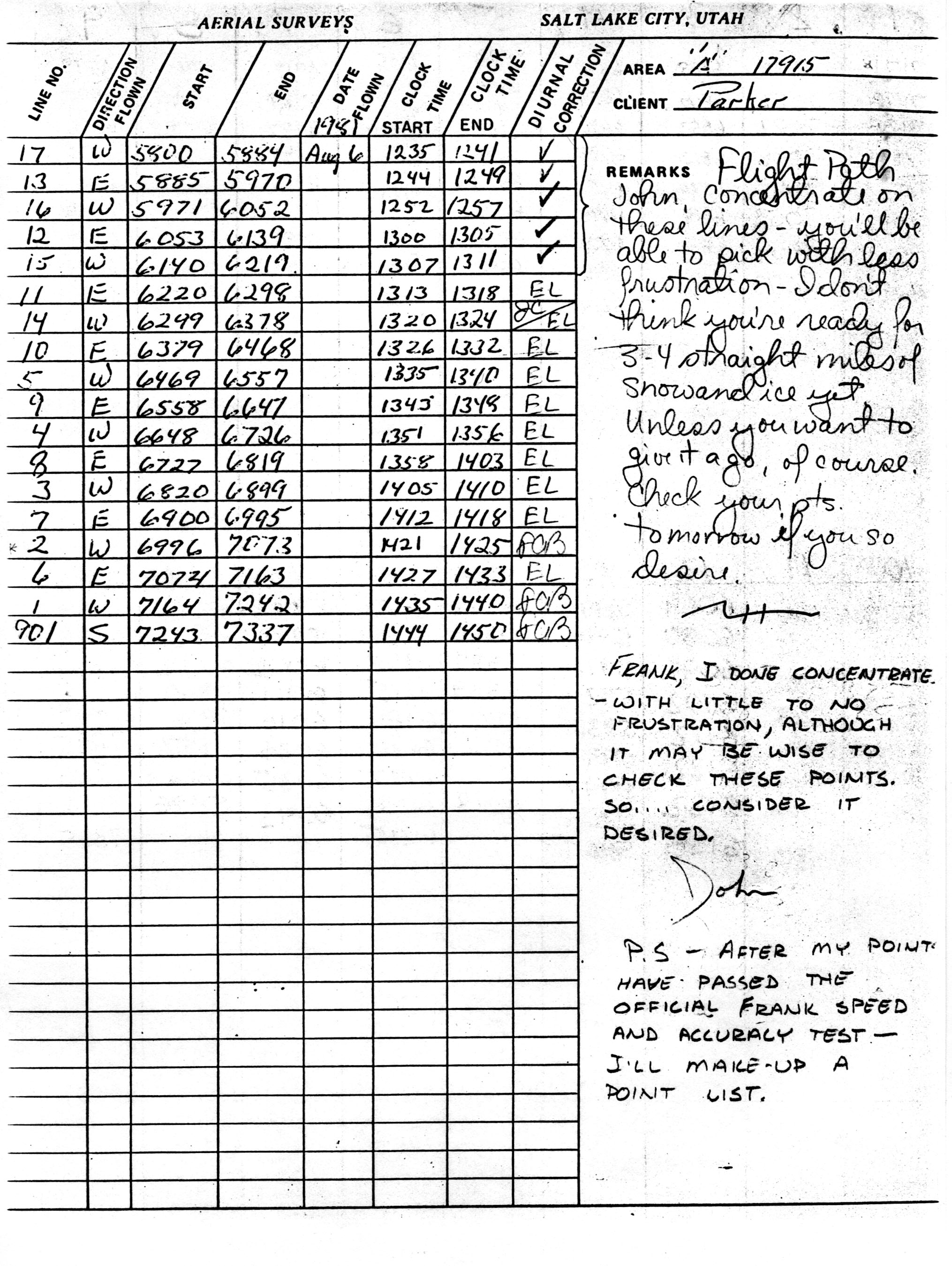
Below is an example of the flight information given to an analyst to use
in the video/ground location reconciliation.
 Click
on image to view larger version
Click
on image to view larger version
![]()
With the use of real-time differential GPS data and pre-programmed flight lines to assist in pilot navigation, the positional accuracy is now about 2-3 meters in horizontal position and 15 meters in vertical position (Denham and Gunn, 1997). Differential GPS navigation has decreased location related errors to less than 2 nano-Tesla (Grauch and Millegan 1998). Modern magnetometers have a resolution of 0.01 nano-Tesla and can cycle every 0.1 second which corresponds to approximately one sample every 5-7 meters on the ground (Denham and Gunn, 1997). New survey designs with relatively close line spacing (< 500 meter) and low flight elevations (< 350 meters draped above the terrain) resolve low-amplitude, short-wavelength magnetic anomalies (Grauch and Millegan, 1998). Although very high resolution surveys are now commonly flown in flat terrain, this type of survey is not commonly done over rugged, highly magnetic terrain such as at Mt. Rainier.
Problems can still exist with these
next generation surveys if the appropriate GPS receiver and datum shifts
are not applied before modeling the magnetic data. In this survey,
a single channel GPS navigation system was used which resulted in uncertainties
in elevations of the magnetometer of 50-100 m. This error is not
acceptable given the 75 meters of terrain clearance for the flight path.
Therefore, we added the radar elevations, which have resolutions of approximately
25 m, to a digital elevation model accurate to approximately 10 m to generate
the flight height. In addition, the flight lines were flown relative
to the topographic maps which are based on the NAD27 geodetic datum while
the GPS uses WGS84. These shift parameters are -8m (dx), -160m (dy)
and 176m (dz).
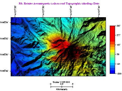
Elevation approximately 150 m draped over terrain. Line spacing approximately 250 m apart.
The low altitude and tight line spacing results in a high
resolution survey. This means that smaller areal extent magnetic anomalies
can be seen in the resulting grid. Instead of picking up general patterns
of magnetic anomalies, we can resolve variable magnetization within the
edifice. In particular, magnetic lows associated with alteration can be
observed. The results can be quite different than the image generated from
the old surveys (Finn, et al., 1998, 1999).
Resulting image from 1996 Mt. Rainier flight:
 Click
on image to view larger version
Click
on image to view larger version
Reduced-to-the-pole magnetic data represented in grid form, draped over topography.
We reduced the observed magnetic data to the pole, a technique
that attempts to account for the inclination of the Earth's magnetic field.
Its principal effect is to shift magnetic anomalies to positions directly
above their sources (Baranov and Naudy, 1964). The red areas correspond
to magnetic, normally-magnetized, fresh dacitic-andesitic rocks not demagnetized
by weathering or hydrothermal activity. Blue colors represent lows caused
by topography and demagnetized volcanic rock.
![]()
Also trailing behind the helicopter
was an electromagnetic (EM) bird. The transmitter and receiver coils in
the EM bird measure the electromagnetic response of the ground at different
frequencies to obtain information from different depths. The raw
data is processed to produce apparent resistivity maps. The deepest that
the lowest frequency EM data can penetrate the surface at Mt. Rainier is
about 150 m beneath the ice. Unlike the magnetic data, the EM is
not very influenced by topography. Altered volcanic rocks produce
lows on resistivity maps, whereas fresh volcanic rocks produce highs.
Ice is very resistive, forming highs (reds) on the images.
 Click
on image to view larger version
Click
on image to view larger version Click
on image to view larger version
Click
on image to view larger version
 Click
on image to view larger version
Click
on image to view larger version
 Click
on image to view larger version
Click
on image to view larger version
![]()
![]()
Denham, D., and P.J.E. Gunn, 1997, Airborne geophysics in Australia; the government contribution, Airborne magnetic and radiometric surveys, AGSO Journal of Australian Geology and Geophysics, 17 (2), 3-9.
Finn, C., Sisson, T.W. and M. Descsz-Pan, 1999, Estimates of volumes and distribution of altered zones on Mt. Rainier with Aerogeophysical data [abs], EOS, Transactions, supplement to November 16, 1999, V32B-04.
Finn, C., Descsz-Pan, M. and V. Rystrom, 1998, Hunting for volcanic weakness at Mt. Rainier with aerogeophysical data [abs], EOS, Transactions, v. 79, p. F978.
Finn, C., and D.L. Williams, 1987, An aeromagnetic study of Mount St. Helens, Special section on Mount St. Helens, Journal of Geophysical Research, B, Solid Earth and Planets, 92 (10), 10,194-10,206.
Flanagan, G., and D.L. Williams, 1982, A magnetic investigation of Mount Hood, Oregon, Journal of Geophysical Research B, 87 (4), 2804-2814.
Grauch, V.J.S., and P.S. Millegan, 1998, Mapping intrabasinal faults from high-resolution aeromagnetic data, Leading Edge (Tulsa, OK), 17 (1), 53-55.
U.S.G.S, 1982, Mt. Rainier 1981 Aeromagnetic Survey, Open File Report: OF 82-0547.
![]()