
Digital Mapping Techniques '01 -- Workshop Proceedings
U.S. Geological Survey Open-File Report 01-223
3D Geologic Maps and Visualization: A New Approach to the Geology of the Santa Clara (Silicon) Valley, California
By R.C. Jachens1, C.M. Wentworth1, D.L. Gautier1, and S. Pack2
1U.S. Geological Survey
345 Middlefield Road, MS 989
Menlo Park, CA 94025
Telephone: (650) 329-5300
Fax: (650) 329-5133
e-mail: jachens@usgs.gov
2Dynamic Graphics, Inc.
1015 Atlantic Avenue
Alameda, CA 94501-1154
Telephone: (510) 522-0700
Fax: (510) 522-5670
e-mail: skip@dgi.com
ABSTRACT
The USGS recently began a long-range project to construct a 3D geologic map of the Santa Clara ("Silicon") Valley, southern San Francisco Bay area, California. This is part of a larger project that also involves developing techniques for constructing 3D models, defining uncertainties associated with geologic elements and properties, and designing procedures for visualizing, accessing, and releasing 3D geologic information. This multipurpose map is intended to provide a quantitative basis for modeling processes including groundwater flow, contaminant dispersion from naturally occurring mercury and asbestos, ground shaking, seismic wave propagation, and tectonic strain accumulation. The fundamental map architecture is defined by critical surfaces (faults, intrusive contacts, unconformities, other depositional contacts) interacting to form volumes, which ultimately are assigned measurement-based properties according to geologic identity, geometric position, or both. Quantitative definition of critical surfaces is based mainly on surface geology, drillhole data, cone penetrometer testing, gravity and magnetic modeling, seismic reflection and refraction profiling, and earthquakes. Critical surfaces are assembled into a 3D map using earthVision (Dynamic Graphics, Inc.) modeling software.
The map volume is 45X45 km by 14 km deep, and spans the valley floor and surrounding hillsides between the San Andreas and Calaveras faults. It is divided by 11 major faults into blocks, within which the Cenozoic section is represented by up to three layers, and the Mesozoic section by more than six units. The 3D map exists in the computer as 1) a set of numerical grids (large cell raster datasets) that quantitatively define the positions and shapes of the critical surfaces, 2) a set of instructions that specify how these surfaces interact when they encounter each other, and 3) the software to assemble the surfaces according to the specified instructions and to assign properties to the map volume. The present 3D map includes the fundamental geometry, architecture, and interaction instructions, though many of the surfaces are as yet only approximately defined. This framework allows us to progressively refine the individual surfaces in an iterative fashion without altering the fundamental model architecture.
INTRODUCTION
Computer-based representations of areal geology extended into the subsurface as 3-dimensional geologic maps can now be developed to provide continuous quantitative 3-D geologic information for a variety of practical needs. Such 3D databases and appropriate computer software will allow even the inexperienced user to figuratively "walk around" in the earth to examine the data and extract needed information. One important application unique to 3D geologic maps is predictive process modeling of geologic, tectonic, and hydrologic processes needed for land-use planning, hazard mitigation, and resource management. Examples of immediate applications of 3D maps include ground shaking estimation, refined earthquake relocation, fault segmentation analysis for probabilistic earthquake forecasting, resource exploration, contaminant source and dispersion pathway definition, and ground water flow modeling for resource management.
Traditional geologic maps, which show the distribution and orientation of geologic materials and structures at the ground surface, have served for many decades as effective tools for storing and transmitting geologic information. The introduction of Geographic Information Systems (GIS) enhanced traditional geologic maps in terms of ease of use and communication of surface geologic information. However, these maps, even enhanced with GIS capabilities, are insufficient for storing and transmitting subsurface information, information that is critical in the role of the map as a window into the subsurface. Fortunately, advances in computer hardware and geologic modeling and visualization software now provide us with the potential to construct 3D geologic maps that retain all the information in a traditional geologic map while quantitatively extending this information into the subsurface. This year the U.S. Geological Survey launched a project titled 3-Dimensional Geologic Maps and Visualization that is designed to take the strong Survey background in the production of traditional geologic maps to the next level by explicitly adding the third dimension.
The goal of the project is to produce, display, and release quantitative 3-dimensional geologic maps, initially in the San Francisco Bay region. The 3D maps will include, in a continuous quantitative volumetric format, the information contained in traditional 2D geologic maps and thus can form the bases for predictive process modeling as well as address, in 3-dimensions, traditional geologic map-based questions. A critical component of these 3D maps will be the inclusion of a continuous representation of uncertainties, a feature only partly realized in traditional geologic maps. Fundamental techniques peculiar to 3D map generation will be developed to accomplish this goal.
3D GEOLOGIC MAP ARCHITECTURE
The 3D maps, which are being designed and constructed under this project are framed around the earthVision geologic modeling and visualization software, retain the fundamental architecture of traditional geologic maps while extending it into the third dimension. Lines on a 2D geologic map (e.g. faults, intrusive contacts, depositional contacts, etc.) become surfaces, and areas transform into volumes in 3 dimensions.
We follow a rigorous sequence of procedures in constructing our 3D geologic maps. First, point data representing discrete 3D locations on a given geologic surface (e.g. a fault) are assembled from surface geologic mapping, well data, geophysical inversions, seismicity, geologic reasoning, and any other sources available. A numerically defined surface is then passed through these data points in order to predict the position of the geologic surface throughout the 3D map volume. Uncertainty as a function of position is assigned to each surface. Once all important surfaces have been defined in this way, they are assembled into a 3D structure according to "rules" that specify how the surfaces interact (i.e., which surfaces truncate which). The surfaces, together with the interaction rules, define volumes that correspond to fault blocks and geologic units. Properties are then assigned throughout the 3D geologic map according to xyz location, geologic identity, proximity to surfaces, geologic process model considerations, or some combination of these parameters. Thus the 3D geologic map exists in the computer as a collection of numerically defined surfaces with associated uncertainties, a set of rules that specify spatial interactions where surfaces encounter each other, and a volume distribution of properties with associated uncertainties. Note that because the map is numerical, it is capable of an enormous dynamic range when defining features. Theoretically, strata a few cm thick could be faithfully included in a geologic map that extends through the entire earth's crust.
Once the 3D map has been assembled within the computer, graphical representations (e.g. figs. 1, 2) permit the user to examine the map from various directions, slice it to examine its interior, disassemble it to examine individual geologic units, compare it graphically with other geographically defined data, and perform a number of other tasks. While graphical representations are valuable tools with which to make use of the 3D geologic map they are simply graphical extracts from the real 3D geologic map that exists digitally within the computer.
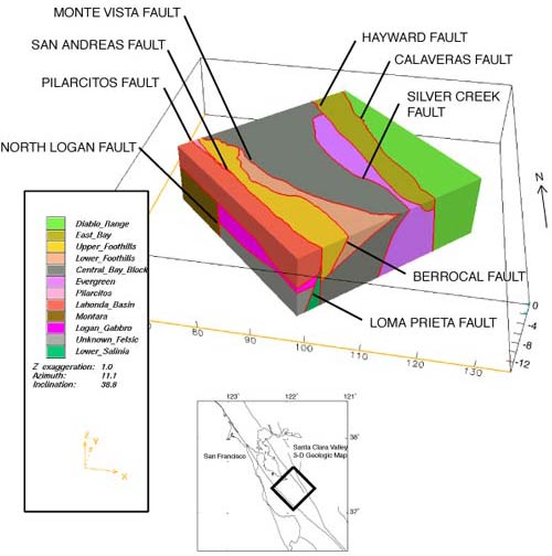
Figure 1. Fault block diagram of the Santa Clara Valley 3D geologic map. Map volume is divided by 11 major faults. Fault surfaces shown are only approximate representations of the actual fault surfaces, and have been assembled to show the fault block architecture of the 3D map. No vertical exaggeration.
|
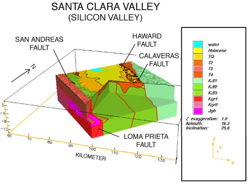
Figure 2. Simple 3D geologic map of the Santa Clara Valley and surrounding hillsides. Only gross geologic units and approximate geologic surfaces are shown. Block has been "chair" cut to reveal some internal geologic information. Topographic surface derived from the 30 m digital elevation model (DEM) of the San Francisco Bay region. No vertical exaggeration.
|
DATA SOURCES
One of the constraints we have imposed on this project is that the tools, techniques, and 3D geologic maps developed here must be based on the types of data that typically would be available. In our map areas, we cannot necessarily expect to have 3D seismic surveys, detailed high-density drill-hole arrays, or similar data sets on which the exploration industries generally base their site-specific 3D geologic models. Furthermore, in most cases we will need to work with data that were collected for other purposes. The types of data that might generally be available are:
Geologic Maps
In most areas, geologic maps of the ground surface provide the scientific and conceptual framework for the 3D geologic map, and constitute one of the most complete data sets in terms of areal coverage. The surface maps identify the geologic units and the major structures that must be included in the 3D map, and the relationships among these units and structures. The geologic and tectonic history inferred from the map will guide many of the decisions that will be needed to specify the geologic units and structures everywhere in the subsurface. Finally, the maps include quantitative point data for constraining the location and shape of critical surfaces, and background information for characterizing properties associated with geologic materials.
Well Data
Data from drill-holes are generally the most important source of point data for defining the locations of critical surfaces in the subsurface. It is possible that a number of different well data sets may be available. These might include:
- water wells, with associated driller's logs and, occasionally, geophysical logs
- geotechnical wells from large construction projects or groundwater contamination
- investigations, which tend to be shallow but often have detailed lithologic and geophysical logs miscellaneous wells such as those drilled during exploration for natural resources (hydrocarbon, geothermal, or mineral resources).
Seismic Profiles
Seismic reflection and refraction profiles and their interpretations provide important 2D subsurface information along profiles and provide critical links between subsurface physical property boundaries and geologic structures and contacts mapped at the surface. If properly placed, they can be used to integrate well data with surface geology and to define the subsurface locations of critical surfaces between points determined from well data.
Typical sources of seismic profile data include university and U.S. Geological Survey scientific investigations of the Earth's crust, seismic reflection surveys for oil and gas exploration, and shallow seismic studies in support of large construction projects and groundwater basin evaluations. Areas that include large water masses such as bays, large lakes, and open oceans along the coasts, often contain marine seismic reflection profiles collected for exploration or hazard mitigation purposes.
Electrical Sounding and Profiles
Vertical electrical soundings based on direct current resistivity measurements or controlled source electromagnetic measurements provide point or 2D information on the subsurface distribution of electrical properties. These data, combined with electrical and geologic data from wells, can be used in a manner similar to seismic profiles, i.e., to define 2D positions of geologic interfaces in the subsurface. However, caution should be exercised in the use of these data because unambiguous correlation of electrical properties with geologic features is challenging.
Electrical sounding and profile data typically are collected in support of ground water investigations and engineering studies. Some data may be found in areas with geothermal resource potential.
Seismicity
In seismically active regions, the 3D locations of earthquakes (hypocenters) can provide unique information on the subsurface shape and location of active faults. Such faults tend to be major structures in 3D geologic maps. Modern methods used to locate earthquakes (Ellsworth and others, 2000) produce distributions of hypocenters that, in some cases, define curviplaner features with surface areas measured in hundreds of km2, yet fault-normal thicknesses of a few hundred meters or less (fig. 3). Few techniques, other than drilling and seismic reflection profiling, provide such accurate subsurface information.
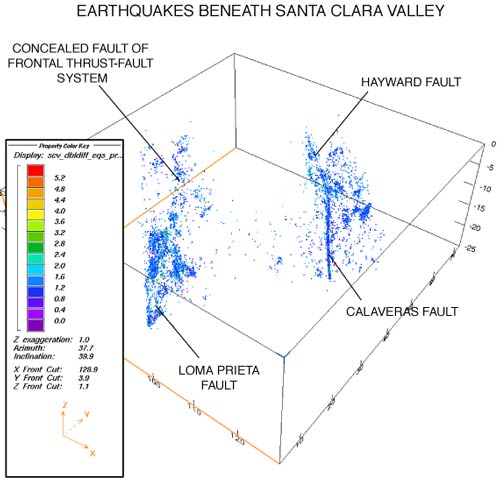
Figure 3. Earthquakes (1984-2000) within the Santa Clara Valley 3D geologic map. Volume is aligned to permit sighting northwest along the seismicity occurring on the Calaveras fault. Other clusters of seismicity associated with faults are identified, including an elongate distribution that we speculate occurs on a concealed, outboard member of the frontal thrust-fault system that bounds the southwest edge of the Santa Clara Valley. No vertical exaggeration.
|
Gravity and Magnetic Map Data
Maps of gravity and magnetic anomalies (figs. 4, 5) are available for most of North America and much of the rest of the world. These maps reflect the subsurface variations of rock density (gravity anomaly) or rock magnetization (magnetic anomaly), properties that often can be related to rock type. Any gravity or magnetic anomaly produced by a subsurface geologic body contains quantitative information about the size, shape, and subsurface location of the source body. The information is ambiguous, however, because a gravity and/or magnetic anomaly does not uniquely define its source. Quantitative interpretation of gravity and magnetic anomalies within constraints provided by geology, well data, other geophysical interpretations, and physical reasoning can be effective in reducing the ambiguity.
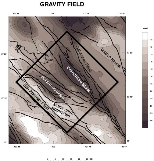
Figure 4. Map showing the residual gravity field of the Santa Clara Valley and vicinity. The gravity field, in conjunction with mapped geology, drill hole data, seismic profiling, and other geophysical interpretations, is used to infer the location and shape of the contact between the Cenozoic deposits and the underlying Mesozoic bedrock. This interface, which tends to be a strong density contrast in the Santa Clara Valley, shows considerable relief, especially in the Cupertino and Evergreen basins. Heavy rectangle is map view outline of the 3D geologic map of the Santa Clara Valley. Faults after Jennings (1994). Contour interval, 5 mGal.
|
Figure 5. Map showing the residual magnetic field of the Santa Clara Valley and vicinity. The magnetic field is used to define the shape and location of the buried Logan Gabbro southwest of the San Andreas fault, and various serpentinite (designated by "S") and metavolcanic bodies northeast of the fault. Heavy rectangle is map view outline of the 3D geologic map of the Santa Clara Valley. Faults after Jennings (1994). Contour interval, 25 nanoTesla.
|
Because gravity and magnetic anomaly data typically will cover the entire area of interest (2D map format), yet reflect the geology of the subsurface, one of their most useful roles is as an interpolator between other scattered data. For example, a subsurface density boundary (e.g. the contact between crystalline basement rocks and overlying Cenozoic sedimentary deposits) might be known in a few locations where penetrated by wells, be known from surface mapping as an exposed contact, and be imaged along an isolated seismic reflection profile. Gravity anomaly data provide a basis for connecting the isolated point data with a spatially continuous 3D surface representing this contact. Magnetic anomaly data can be used in a similar fashion to define 3D surfaces separating geologic bodies with different magnetic properties. In still other cases, the gravity and magnetic data may be interpreted nearly independently to produce 3D representations of the geology and structure of the subsurface.
Other Data
The foregoing data types are typically the most readily available, although on occasion other types of data such as seismic tomography, magnetotelluric soundings, geochemical sampling, or hydrologic modeling, might be used to help construct a 3D geologic map. When viewed in the context of trying to define the geologic map everywhere in the subsurface, the distribution and number of these data seem extremely limited. They are almost never dense enough to support direct geospatial modeling of the type used in mining exploration or ground water contamination remediation investigations. Therefore, in order to construct a fully 3D geologic map from these types of data, it is necessary to develop tools with which to make better use of the data.
TOOLS FOR CONSTRUCTING QUANTITATIVE 3D GEOLOGIC MAPS
Projecting Geology Quantitatively into the Subsurface
Geologic maps portraying the geology at the ground surface typically constitute one of the most detailed and extensive data sets available for constructing quantitative 3D geologic maps. New techniques are needed, however, for projecting this geology into the subsurface and defining the uncertainties associated with the projection of various geologic entities. As an initial effort, we are developing an interactive computer-based system that will facilitate the generation of geologic cross sections which then can be linked by "tie-lines" to produce a 3D map (Fitzgibbon and others, 2001).
3D Inversion of Gravity and Magnetic Data
Gravity and magnetic anomaly maps contain quantitative information about the distribution of density and magnetization contrasts contained within the crust, and often these physical property distributions can be related directly to geology (Blakely, 1995). For example, in the Santa Clara Valley much of the character expressed in the gravity anomaly field is attributable to variations in the thickness of Cenozoic deposits overlying Cretaceous and older bedrock. Similarly, more than 90% of the magnetic anomalies reflect exposed and concealed tabular bodies of serpentinite or metavolcanic rock. Defining these geologic elements in 3 dimensions will go a long way toward building a good 3D geologic map of the Santa Clara Valley. In particular, the serpentinite bodies not only make up a significant part of the pre-Cenozoic rock beneath the Santa Clara Valley, but they often lie within, and thus define, fault zones cutting the pre-Cenozoic bedrock.
For this project, we have begun by evaluating existing techniques for the 3D inversion of gravity and magnetic anomalies, and developing an inversion technique specifically designed to determine quantitatively the 3D location and shape of tabular magnetic bodies in the subsurface. We are also experimenting with the application of gravity inversion techniques to magnetic inversions through the use of the pseudogravity transform (Baranov, 1957).
Smart Interpolation Techniques
To be successful in constructing a useful 3D geologic map from incomplete or sparse data, techniques are needed for defining the positions of the surfaces between control points that are "smarter" than simply connecting the control points with lines or planes. Two general categories are 1) those that use remotely sensed data containing somewhat ambiguous information about the surface to constrain the shape of a given concealed surface between control points, and 2) techniques that use geologic principles and models to interpolate between control points.
In the first category, we are refining a procedure that uses surface gravity observations to infer the 3D position of a concealed density interface (e.g. the contact between the Cenozoic and pre-Cenozoic rocks beneath the Santa Clara Valley) subject to constraints from surface geology, well penetrations, and other geophysical interpretations (Jachens and Moring, 1990). We also are examining uncertainties associated with this inversion, especially in terms of the observed gravity and assumed subsurface density distributions. In the second category, we are looking toward utilizing the extensive developments that have taken place within the petroleum-related sciences related to the application of sedimentological models, diagenetic concepts, sequence stratigraphy principles, balanced cross section analyses, etc., and their possible applications to the construction of 3D geologic maps. In particular, we are looking to the petroleum-related sciences for techniques that can be used with water well log data to generate 3D geologic maps of the upper few hundred meters of the crust.
Statistical vs. Deterministic Representations of Geology and Rock Properties
For some processes and at some scales, statistical representations of geology or rock properties may be more appropriate than deterministic representations. For example, estimating the total storage capacity of an aquifer or the total amount of water that might be extracted before subsidence and fissuring become a problem could be cases where statistical representations of hydrogeologic properties are adequate. We have not yet strayed from our intent to construct a deterministic 3D geologic map of the Santa Clara Valley, but the availability of a small number of volumetrically restricted but intensely studied contamination sites could provide the data for such a statistical representation of a part of the subsurface.
3-DIMENSIONAL GEOLOGIC MAP OF THE SANTA CLARA VALLEY: PRESENT STATUS
The 3D geologic map of the Santa Clara Valley is still in its infancy, due to the fact that the project is only about 8 months old, large data compilation efforts are required before the map can be generated, and many of the tools needed to construct the map are not available and are not simple to develop. Nevertheless, progress has been made, and the preliminary 3D map, while crude, already is providing fascinating insights into some important geologic problems.
Current Map
Our major map-related accomplishment has been the definition of the fundamental 3D architecture of the Santa Clara Valley 3D map, and the construction of a "strawman" map populated with rough approximations or surrogates of the surfaces that will be needed in the final map (figs 1, 2). Details of the "strawman" are based mostly on new geologic compilations (Graymer and others, 1996; Brabb and others, 1998; Wentworth and others, 1998), inferences from gravity and magnetic anomalies (figs. 4, 5), seismicity (fig. 3), and limited well information. The map exists in the computer as a set of digital grids that define the critical geologic surfaces in 3 dimensions, and a set of instructions in earthVision that specify how the surfaces interact when they encounter each other (i.e. which surfaces truncate which). This digital map is represented in the flow diagram shown in figure 6, and the block diagrams of the map shown in figures 1 and 2 can be thought of as cartographic representations of the digital map. The map volume is divided into fault blocks by 11 major faults, some of which are active today (fig. 1). At present, each fault block includes no more than five major geologic units (fig. 2), although future versions will include more complexity.
Figure 6. Schematic representation of the Santa Clara Valley 3D geologic map. This schematic defines the fault-block structure and the geologic units that make up the 3D geologic map. The map is composed of:
- surfaces (faults, contacts, etc.) defined by numerical grids (e.g. scv_dem30_prj_mod.2grd)
- rules governing how the surfaces interact where they meet
- volumes bounded by multiple surfaces
- properties assigned to volumes
FAULT TREE -- gives the arrangement of faults that divide the map into fault-blocks. Placement of a fault in the tree structure determines its relation to other faults. A given fault truncates against all faults to its left.
GEOLOGIC SEQUENCE -- gives the arrangement of geologic units within a fault-block. Placement of a unit in the vertical stack determines its relative location in the vertical dimension of the map, and the geologic relations (deposition, unconformity, channel erosion) control how the bounding surfaces interact where they meet.
|
The present 3D map is in a flexible format that permits refinement without disrupting its fundamental architecture, and, further, allows existing scientific questions to be addressed before the map is completed. Progressive refinement can and will take place surface by surface. Whenever a specific geologic surface (e.g. the San Andreas fault) is better defined, we simply replace the surrogate digital grid in the computer with our new grid, activate the geologic-structure-building software, and produce a refined version of the 3D geologic map. Individual fault blocks or geologic units can be subdivided by additional faults and/or contacts without disrupting other fault blocks or geologic units simply by adding new surfaces and interaction instructions, and again activating the geologic-structure-building software. We currently are focussing efforts on refining those fault surfaces that are reflected in the seismicity (San Andreas, Calaveras, and Hayward faults, and elements of the Monte Vista fault zone) and on the contacts that mark the bases of the Holocene and Tertiary deposits.
Current Science
The present 3D geologic map of the Santa Clara Valley, even in its crude, approximate state, already is providing insights into some scientific questions by facilitating the comparison of different data sets within a coherent 3D framework. This is particularly true of comparisons between seismicity and 3D geology.
Seismicity triggered by the 1989 Loma Prieta earthquake occurred in the region northwest of the primary aftershock region (labeled "concealed fault of frontal thrust-fault system" in figure 3). In our model, this corresponds to the northwest half of the map (fig. 2) along the San Andreas fault, in the region immediately northeast of the fault. Examining this triggered seismicity within the 3D geologic map suggests that it occurred along a low-angle, southwest-dipping fault that roots in the San Andreas fault at depths of 7-8 km. Toward the northeast the fault terminates beneath the Santa Clara Valley where it intersects the top of buried Mesozoic bedrock (the base of the Tertiary deposits T2 in figure 2). The seismicity could be occurring on a concealed, basinward member of the southwest-dipping frontal thrust-fault system (McLaughlin and others, 2000) represented by the Berrocal and Monte Vista faults (fig. 1). This fault could pose a direct hazard to the Santa Clara Valley.
The shape of the Mesozoic bedrock surface beneath the Santa Clara Valley indicates a deep Cenozoic basin along its southwest edge that could contain as much as 4-5 km of Cenozoic deposits. This inference is based on inversion of the gravity data but has not been confirmed by deep drilling, seismic profiling, or any other direct methods. However, recent studies of oil extracted from wells and seeps along the southwest edge of the Santa Clara Valley indicates that the oil originated in the Miocene deposits and matured at minimum depths of 2-3 km (Stanley and others, 1996). Thus, the preliminary 3D geologic map provides a possible explanation for the origin of oil seeps in the Santa Clara Valley, whereas the studies of the oil itself provide indirect confirmation of the existence of a deep basin beneath the valley.
The mainshock of the 1989 Loma Prieta earthquake and many of its aftershocks have occurred along a southwest-dipping plane that lies close to, but southwest of, the mapped trace of the San Andreas fault. Some researchers have argued that the earthquake was not on the San Andreas fault proper (e.g. Segal and Lisowski, 1990), but no consensus has been reached. In the present 3D geologic map (figs. 1,2), the lower half of the fault block southwest of the San Andreas fault is divided by the North Logan Fault (fig. 1), a fault inferred from the aeromagnetic data (fig. 5) to lie along the straight northern boundary of the concealed magnetic Logan Gabbro. The magnetic anomaly implies that the fault is about 40 km long, cuts across the entire block between the San Andreas fault and the San Gregorio fault to the west, but does not offset the San Andreas fault (Jachens and others, 1998). Thus, these data suggest that the North Logan fault is confined entirely to the block southwest of the San Andreas fault. Interestingly, the southwest-dipping Loma Prieta aftershock distribution lies only south of the inferred North Logan fault and terminates (farthest northwest extent) at the inferred location of the North Logan Fault. We argue that the spatial coincidence of the dipping Loma Prieta aftershock distribution with geologic units and structures confined to the fault block southwest of the San Andreas fault supports the interpretation that the Loma Prieta earthquake occurred on a fault within the southwestern block and not on the San Andreas fault itself.
FUTURE PLANS
This project is still in its infancy, but initial results are extremely encouraging. We plan to continue building the 3D geologic map by addressing a wide range of tasks. These include surface geologic mapping to address specific problems, analysis of well information, constrained inversion of geophysical data, analysis and application of sedimentological models, development of new tools for improved use of the available data, and development and evaluation of effective methods for visualization and distribution of 3D geologic maps. These tasks are difficult and complex, and we realize that we may not fully succeed in completing them. Our experience to date, however, gives us confidence that we will be able to construct a 3D geologic map of the Santa Clara Valley that will significantly improve upon such information as is currently available. In the meantime, we will capitalize on the evolving 3D map to support our scientific investigations.
REFERENCES CITED
Baranov, V., 1957, A new method for interpretation of aeromagnetic maps: Pseudo-gravimetric anomalies: Geophysics, v. 22, p. 359-383.
Blakely, R.J., 1995, Potential theory in gravity and magnetic applications: Cambridge University Press, 441 p.
Brabb, E.E., Graymer, R.W., and Jones, D.L., 1998, Geology of the Palo Alto 30 X 60 minute quadrangle, California: a digital database: U.S. Geological Survey Open File Report 98-348.
Ellsworth, W.L., Beroza, G.C., Julian, B.R., Klein, F., Michael, A.J., Oppenheimer, D.H., Prejean, S.G., Richards-Dinger, K., Ross, S.L., Schaff, D.P., and Waldhauser, F., 2000, Seismicity of the San Andreas fault system in central California: Application of the double-difference location algorithm on a regional scale: Eos, Transactions, American Geophysical Union, v. 81, p. F919.
Fitzgibbon, T.T., Phelps, G.A., and Jachens, R.C., 2001, GIS tools for the construction of 3D geologic models: Geological Society of America Abstracts with Programs v. 33, p. A-40.
Graymer, R.W., Jones, D.L., and Brabb, E.E., 1996, Preliminary geologic map emphasizing bedrock formations in Alameda County, California: a digital database: U.S. Geological Survey Open File Report 96-252.
Jachens, R.C., and Moring, B.C., 1990, Maps of the thickness of Cenozoic deposits and the isostatic residual gravity over basement for Nevada: U.S. Geological Survey Open-File Report 90-404, 15 p., 2 sheets, scale 1:1,000,000.
Jachens, R.C., Wentworth, C.M., and McLaughlin, R.J., 1998, Pre-San Andreas location of the Gualala block inferred from magnetic and gravity anomalies, in Elder, W.P., (ed.), Geology and tectonics of the Gualala block, northern California: The Pacific Section, SEPM, Society of Sedimentary Geology, Book 84, p. 27-64.
Jennings, C.W., 1994, Fault activity map of California and adjacent areas, with locations and ages of recent volcanic eruptions: California Division of Mines and Geology California Geologic Data Map Series 6, scale 1:750,000.
McLaughlin, R.J., Langenheim, V.E., Schmidt, K.M., Jachens, R.C., Stanley, R.G., Jayko, A.S., McDougal, K.A., Tinsley, J.C., and Valin, Z.C., 2000, Neogene contraction between the San Andreas fault and the Santa Clara Valley, San Francisco Bay Region, California, in Ernst, W.G., and Coleman, R.G., (eds.), Tectonic studies of Asia and the Pacific rim: Geological Society of America, International Book Series, v. 3, p. 265-294.
Segall, P. and Lisowski, M, 1990, Surface displacements in the 1906 San Francisco and 1989 Loma Prieta earthquakes: Science, v. 250, p. 1241-1244.
Stanley, R.G., Jachens, R.C., Kvenvolden, K.A., Hostettler, F.D., Magoon, L.B., and Lillis, P.G., 1996, Evidence for an oil-bearing sedimentary basin of probable Miocene age beneath "Silicon Valley", California: annual Meeting Abstracts-American Association of Petroleum Geologists and Society of Economic Paleontologists and Mineralogists, v. 5, p.133-134.
Wentworth, C.M., Blake, M.C., Jr., McLaughlin, R.J., and Graymer, R.W., 1998, Preliminary geologic map of the San Jose 30 X 60-minute quadrangle, California: a digital database: U.S. Geological Survey Open-File Report 98-795.
RETURN TO Contents
National Cooperative Geologic
Mapping Program | Geologic Division |
Open-File Reports
U.S. Department of the Interior, U.S. Geological Survey
URL: https://pubsdata.usgs.gov/pubs/of/2001/of01-223/jachens.html
Maintained by David R. Soller
Last modified: 18:24:40 Wed 07 Dec 2016
Privacy statement | General disclaimer | Accessibility