Digital Mapping Techniques '02 -- Workshop Proceedings
U.S. Geological Survey Open-File Report 02-370

New Tricks for Old Dogs: A Digital Technique for Producing Mylar Base Maps for Geologic Mapping and Compilation

By Adam S. Read, David J. McCraw, and Geoffrey Rawling

New Mexico Bureau of Geology and Mineral Resources
New Mexico Institute of Mining and Technology
801 Leroy Place
Socorro, NM 87801
Telephone: (505) 835-5753
Fax: (505) 835-6333
e-mail: adamread@gis.nmt.edu

INTRODUCTION

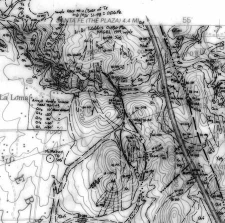
Figure 1. An example of geologic mapping carried out on a traditional photomechanical greenline made from a composite negative of the Seton Village 7.5-minute quadrangle (Read and others, 1999). In this case, the greenline had to be outsourced to a reprographic center capable of photographically enlarging the negative two times to a scale of 1:12,000, to facilitate mapping in an area with a high level of geologic complexity.

PROCESS

Overview

Using a geographic information system (GIS) to produce the digital base makes it possible to add a collar of adjacent topographic maps around the map of interest. It is also possible to include previously mapped geology from these adjacent maps on the new base (Figure 2). This saves time in the field and helps eliminate map boundary mismatches during compilation. A digitally produced base map of a particular area of interest can also circumvent Murphy's first corollary of cartography (that the area of interest generally lies at the intersection of four maps). Also, a UTM grid can easily be added to the map for easier global positioning system navigation. In addition, you can change, remove, or retain the colors used in the original paper topographic base, which can aid in map element recognition (e.g., streams). You can also remove the distracting pattern screens representing forested areas or landownership printed on the original topographic maps. We choose colors that will reproduce using a blueprint machine and are easily differentiated from the black-inked linework. This, of course, greatly simplifies the digital data-capture process -- after the map is compiled by hand, it can be scanned, converted to a paletted image, and rectified in a GIS where the compiled linework can then be turned off for easier digitization.

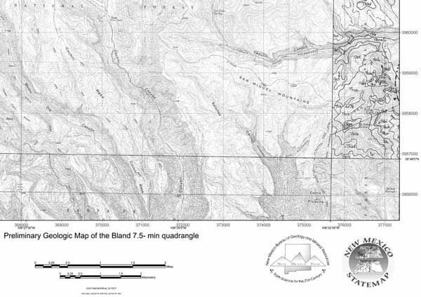
Figure 2. An example of a part of the digitally produced base map of the Bland 7.5-minute quadrangle to be utilized for future geologic mapping. Note that the topography of adjacent quadrangles and the hand-compiled geologic linework of the Frijoles quadrangle (Goff and others, 2001) have been incorporated with the base to facilitate edge-matching.

Process Details

1. Obtain a high-quality 24-bit color scan of the paper topographic base.

   We scan at 400 dpi (the optical resolution of our scanner). We have tried scanning at higher resolutions, but file size becomes an issue and the quality at 400 dpi has been acceptable. A 1:24,000-scale quadrangle scanned at 400 dpi generates a red-green-blue (RGB) tiff file of around 275 Mb.

2. Clean up the image and touch up the green pattern screen of forested areas.

   Adjust the contrast with the Auto Contrast command in Adobe Photoshop and adjust brightness if necessary. Select the green (forested) areas of the map with the magic wand tool in Photoshop with the tool's tolerance set to around 30, and the "contiguous areas," "anti-aliased," and "use all layers" boxes unchecked (see Figure 3). This process with the magic wand tool can take several iterations of holding the shift key down to add to the selection of all of the green pixels. Use a successively lower tolerance to avoid selecting colors representing other map elements. Finally, fill the selected green regions with the standard USGS digital raster graphic (DRG) green. For us, this process has worked best in eliminating the moiré effect from the scanned pattern screen and in separating the green so that we can remove it from the final topographic base.

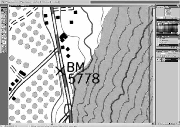
   Figure 3. RGB scan of the Velarde 7.5-minute quadrangle showing the green screen of forest (gray patch) and orchard areas (large gray dots) selected with the magic wand tool in Photoshop. Note that not all of these pixels have been selected yet because both RGB scanning and color variations in CMYK printed paper maps introduce a range of green color values. Several successive selection iterations with the magic wand are often necessary because of the varying hues of green (see text). Once selected, they are filled with the standard USGS DRG green in Photoshop. This step forces the forested areas to be classified as green when converted to the 13-color USGS DRG palette.

3. Convert the RGB image to the USGS standard DRG palette of 13 colors.

   Any palette could be used, but a standard palette of 16 colors or fewer is much easier to work with. We also use clipped versions of the USGS DRGs for the topography of adjacent quadrangles; so using the USGS DRG palette is preferable. We use Adobe Photoshop to palette the image because, of the applications we have tried, it seems to work best. You can easily load this palette into Photoshop by opening a standard USGS DRG and saving the color table. To palette a RGB image, select your custom color table when prompted from the image>mode>indexed color menu. This generates a much smaller tiff file that is about 80 Mb uncompressed. There is apparently an in-house USGS paletting program that does this as well, but we have not been able to obtain it.

4. Rectify the image using ArcMap.

   Rectify the image using all 16 latitude/longitude tics present on the quadrangle (Figure 4). At this point, we decide whether we want to show the topography or geology from adjacent quads on the base map. If so, clip the collar information from the map; if not, proceed to modify the color table.

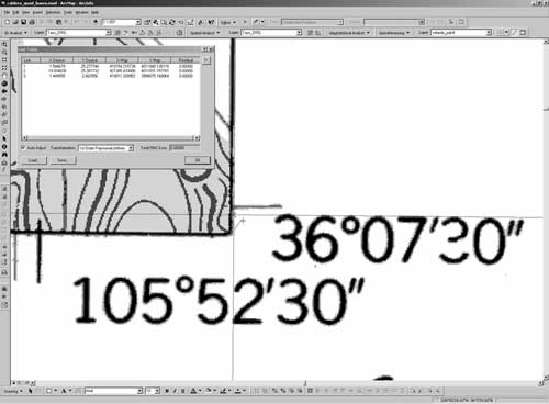
   Figure 4. Rectification process step for the paletted image of the Velarde 7.5-minute quadrangle using ArcMap.

5. Clip the map to the extent of the quadrangle to remove the collar information.

   Reclassify the map to free up the "0" slot in the color table by using the reclassify function of the ArcGIS Spatial Analyst extension to move the black color from the "0" bin to the "13" bin (Figure 5). This step can be combined with the clipping operation if the analysis mask and extent in Spatial Analyst is set to a polygon shapefile or coverage of the quadrangle boundary (obtained from a statewide coverage of 7.5-minute quadrangles). The clipped grid will use the "0" bin for the "no data" area outside the quadrangle, but the clipped grid will no longer retain the original color-table information (Figure 6). Because of a bug in the ArcGIS 8.1.2, it is necessary to do the next step from the ArcInfo command line.

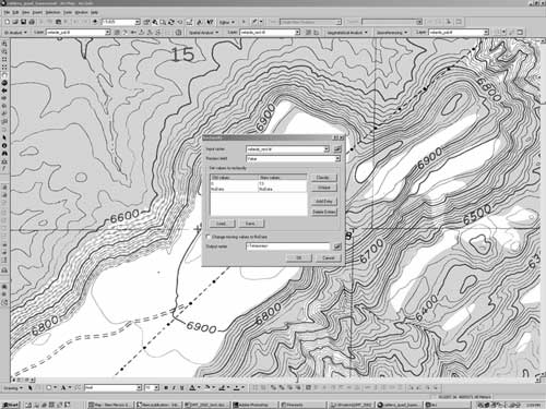
   Figure 5. The reclassification process step for the Velarde 7.5-minute quadrangle in ArcMap. This removes the black color from the "0" bin to free it up for the "no data" area outside the map extent.

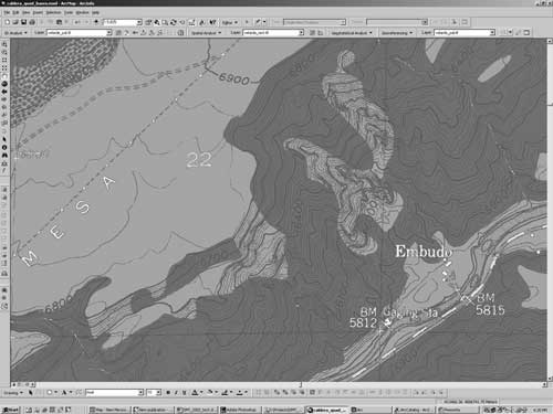
   Figure 6. The clipped grid of the Velarde 7.5-minute quadrangle, which now has no data outside of the quadrangle extent, but has lost the original color-table information.

6. Reintegrate the color table with the clipped image using GRIDIMAGE.

   The first time this step is done, you will need to use the ArcInfo command IMAGEGRID on a reclassified but not clipped image to save the color table to an ASCII file. Use the ArcInfo command GRIDIMAGE to convert the clipped grid to a geotiff raster using the predefined color table (Figure 7).

   Figure 7. The ArcInfo GRIDIMAGE command is used to reintegrate the original color table with the clipped image file.

7. Modify the colors in the color table using ArcMap to make a "greenline" base.
   • Change the black (13) to dark green -- "leaf green" works well.
   • Remove the forested areas' green color (5).
   • Change the contour-line color (4 and 12) to light green -- "fern green" works well.
   • Remove any colors that clutter the image -- gray (11) is sometimes removed.
   • Modify any other colors as necessary -- each quadrangle will need custom color adjustment because the process-color inks used on the paper maps have changed over time.

8. If adjacent quadrangle data are to be included on the map, repeat the previous steps to add it. A similar process can be used to incorporate geology linework from a paletted scan of either a published map or from a hand-drafted mylar. All colors in the palette except the linework can be removed.

9. Add a latitude/longitude graticule and a UTM grid to the map along with scale bar, etc. A red UTM grid will reproduce on a blueprint machine; blue will not.

10. Print the map on paper as a test before trying to print to mylar (Figure 8). (These paper prints are great for field mapping, especially if thin matte mylar is glued to the surface first. We use 3M "Super 77" spray adhesive.)

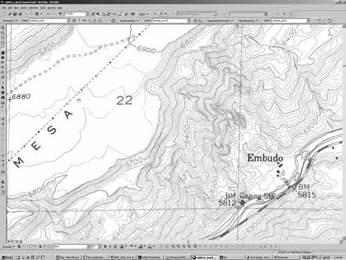
    Figure 8. The digital greenline topographic base for the finished Velarde 7.5-minute quadrangle with the green forested-areas pattern removed and brown contour lines changed to green. The Embudo gaging station on the Rio Grande in the lower right is the oldest continuously active gaging station in the United States, installed by the USGS in 1889.

11. Print a mirror image of the map onto double-matte mylar. This puts the base on the back of the mylar so that hand drafting can be done on the opposite matte side. We use the Postscript driver in ArcMap and set the emulsion side to "down." You could also use the printer driver settings to make a mirror print.

TECHNOLOGY

Software

Hardware

Media

Topographic maps generally look fine with this plotter/media combination. Occasionally, the ink will bleed where there are very close contours or otherwise cluttered areas (monochrome plots look better in these cases). There are many more film-media options if using dye-based inks, but we are concerned that maps plotted with dyes will not be archival documents. Ideally, we would prefer a thicker mylar, perhaps 7 mil, for our larger 1:12,000-scale bases because it would be somewhat more stable. However, no other media has worked as well as the 4-mil Océ media.

CONCLUSION

REFERENCES

McCraw, D.J., 1999, "Can't see the geology for the ground clutter" -- Shortcomings of the modern digital topographic base, in Soller, D.R., ed., Digital Mapping Techniques '99 -- Workshop Proceedings, U.S. Geological Survey Open-File Report 99-386, p. 21-26, https://pubs.usgs.gov/openfile/of99-386/mccraw.html.

Read, A.S., Rogers, J., Ralser, S., Ilg, B., and Kelley, S., 1999, Geology of the Seton Village 7.5-min. quadrangle, Santa Fe County, New Mexico: New Mexico Bureau of Mines and Mineral Resources Open-File Geologic Map OG-GM 23, scale 1:12,000.