
In cooperation with the U.S. Environmental Protection Agency
Figure 1. Location of the three detailed study units and the U.S. Geologica...
Figure 2. Location of the eight study sites for mercury in periphyton, 2003...
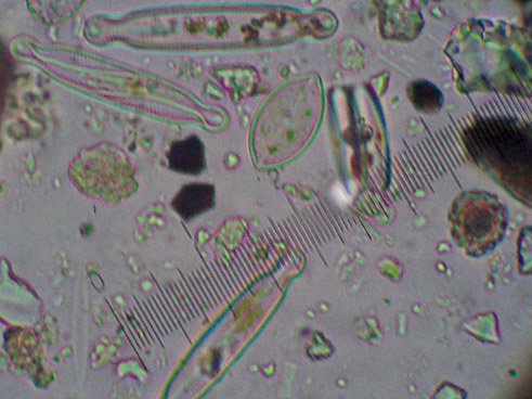
Figure 3. A wide range of algal species at 400X magnification found in the ...
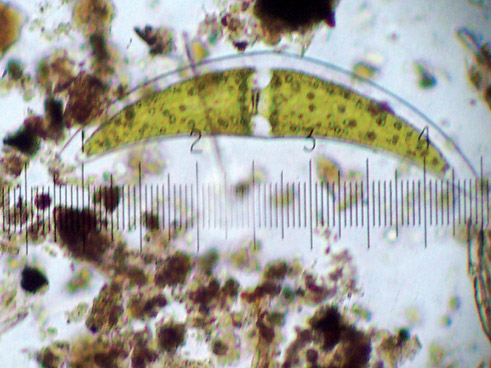
Figure 4. A Chlorophyta (green algae) Closterium sp. at 400X magnification ...
Table 1. Site information for the eight stations sampled for mercury in per...
Table 2. Raw data of all periphyton samples. See table 1 for complete descr...
Table 3. Divisional classification data of all periphyton samples. See tabl...
In aquatic ecosystems, algae are the primary producers and the base of the food web. To date, there has been little research on the role of benthic algae (periphyton) in the bioaccumulation of mercury (Hg) in riverine systems —a key step of the process of bioaccumulation from the physical environment (water and sediments) to higher aquatic organisms (invertebrates, fish, and others). Periphyton has been shown to have an important role in the transfer of mercury in wetlands of the Florida Everglades (Cleckner and others, 1999) and in some situations served as the host site for mercury methylation, which is the key process controlling mercury toxicity in the environment. Pickhardt and others (2002) found that algal blooms in lakes resulted in reduced bioaccumulation of mercury in algal-rich eutrophic lake systems due to decreases in the concentration of mercury per algal cell.
In 2003, the United States Geological Survey (USGS) National Water Quality Assessment (NAWQA) and Toxic Substances Hydrology (Toxics) programs initiated a study to assess mercury bioaccumulation and cycling in eight differing stream-ecosystem settings across the U.S. One aspect of this project involved a detailed examination of the role of periphyton in the trophic transfer of methylmercury (MeHg) in indigenous food webs. This periphyton-mercury study was based in three NAWQA study basins chosen for the first intensive mercury project sampling; the Western Lake Michigan Drainages (WMIC), the Willamette Basin (WILL), and the Georgia-Florida Coastal Plain (GAFL), shown in figure 1. Two to three study sites in each of the three basins were chosen for the NAWQA/Toxics study to represent one urban site and one to two reference/non-cultivated (low- and high-percent wetland) sites. Table 1 lists site information for the sampled rivers, and site locations are shown in figure 2. Currently, there are no generally accepted methods for collection of periphyton for mercury or methylmercury determinations. This paper discusses the collection process and analysis for mercury in periphyton.
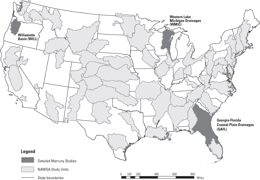
Table 1. Site information for the eight stations sampled for mercury in periphyton, 2003.
[d, degree; m, minute; s, second]
| Study unit | USGS station ID | Station name | River code | Landscape type | Basin area (square miles) | Latitude-longitude (ddmmssdddmmss) | Percent wetland1 |
|---|---|---|---|---|---|---|---|
| GAFL | 02234998 | Little Wekiva River near Longwood, FL | LW | Urban | 44.5 | 2842070812332 | 4.50 |
| GAFL | 02322500 | Santa Fe River near Fort White, FL | SF | Reference, non-cultivated | 1020 | 2950550824255 | 18.0 |
| GAFL | 02231000 | St. Marys River near MacClenny, FL | SM | Reference, non-cultivated | 700 | 3021310820454 | 48.0 |
| WILL | 14206435 | Beaverton Creek at SW 216th Ave, near Orenco, OR | BT | Urban | 36.9 | 4531151225354 | 0.16 |
| WILL | 14161500 | Lookout Creek near Blue River, OR | LO | Reference, non-cultivated | 24.1 | 4412351221520 | 0.00 |
| WMIC | 04075365 | Evergreen River below Evergreen Falls near Langlade, WI | EG | Reference, non-cultivated | 64.5 | 4503570884034 | 9.30 |
| WMIC | 04087204 | Oak Creek at South Milwaukee, WI | OC | Urban | 25.0 | 4255300875212 | 8.10 |
| WMIC | 04066500 | Pike River at Amberg, WI | PR | Reference, non-cultivated | 255 | 4529490881818 | 18.0 |
1 Land use data derived from National Land Cover Dataset using 30-meter Thematic Mapper data (Vogelmann and others, 2001).

Figure 2. Location of the eight study sites for mercury in periphyton, 2003.
Trace-metal clean sampling techniques were used to minimize potential sample contamination (USEPA, 1996; Cleckner and others, 1998; Cleckner and others, 1999). These techniques generally serve to minimize contact between the sample and field crews that employ sampling devices and sample containers that have been stringently cleaned in acid. Prior to use in the field, all glass and Teflon®1 equipment was cleaned by immersing in 4 normal (N) hydrochloric acid (HCl) at 65° celsius (C) for at least 48 hours and then immersed and rinsed at least three times with reagent-grade deionized water (>18 megohms (MOhm)). Equipment other than glass or Teflon® was soaked for at least four hours in a solution of reagent-grade water and Liquinox® (a non-ionic surfactant detergent). This equipment was then triple-rinsed with reagent-grade water, placed in five-percent HCl (Omnitrace) for at least four hours, and finally immersed and triple rinsed with reagent-grade water. After cleaning, all sampling equipment and sample containers were stored by double bagging in hermetically sealed plastic bags.
1 The use of firm, trade, and brand names does not constitute endorsement by the U.S. Government.
At each sampling site, two types of periphyton samples were collected. The (USEPA) Rapid Bioassessment Protocol (Barbour and others, 1999) recommends "single-habitat sampling should be used when biomass of periphyton will be assessed." The single-habitat sampling targets two contrasting habitats that are estimated to be the primary periphyton habitats in the study streams: the depositional-targeted habitat (DTH) and the taxonomically richest-targeted habitat (RTH). The DTH sample may be collected from fine sediment such as silt/clay or sand as appropriate. The DTH and RTH periphyton samples for this study were collected and composited from separate locations in the stream. The NAWQA single habitat sampling method (Moulton and others, 2002) was used for this study because the surface area sampled by this method is quantifiable and those two habitats are generally where periphyton growth dominates in streams.
The overall study design for this project called for seasonal comparison of mercury and methylmercury concentrations and fluxes during spring (high flow) and fall conditions (base flow). For the spring DTH sampling, three areas in each stream were sampled, typically in depositional areas with high organic carbon content in the streambed sediment. These areas were targeted for sampling due to relative abundance of fine sediments and presumably low redox conditions that would promote mercury methylation. Hem (1985) defines redox as the processes of a participating element losing or gaining orbital electrons. The sediment sampling procedure employed by this study seeks to capture the upper 0.5 centimeters (cm) of sediment by employing a Teflon® petri dish (2.54 cm diameter) that is carefully placed open-side down on the streambed sediment to enclose a 19.64 cm2 circle of sediment. A thin sheet of Teflon® was slid under the opening to capture the sediment contained in the petri dish, which is then transferred into a 500 milliliter (mL) Teflon® jar. A more complete description of this method can be found in Porter and others (1993) and Moulton and others (2002) with the addition of trace-metal-clean techniques. For the fall DTH sampling, subsamples were collected at specific areas where methylation rates were found to have the highest methylation potential during the springtime sampling (M. Marvin-DiPasquale, U.S. Geological Survey, Menlo Park, Calif., written commun., August 11, 2003).
The RTH samples were collected from either rock cobbles (epilithic) or woody snags (epidendric) by brushing the algal growth with a stiff-bristled toothbrush-type brush into a Teflon® dish and transferring the slurry into a 500-mL Teflon® jar. Five cobble or woody snags were collected at five locations in each stream for a total of twenty-five composited samples as described in Moulton and others (2002). This method was used with the addition of trace-metal-clean techniques. Rock cobble was the preferred substrate in the WMIC and WILL basins; however, woody snags were used in the GAFL basin because of a general lack of cobble or larger sized rocks at these sites. To determine the surface area of the cobble samples, a section of aluminum foil was placed over the rock and cut to the size and shape of the area scraped. Each sample template was then weighed to determine surface area based on a seven-point curve of mass to surface area from each roll of aluminum foil used. To determine surface area of the woody snags, the length of each snag was measured to the nearest millimeter excluding the first two centimeters from each end. These areas were not scraped to minimize contamination from handling and cutting of the snag.
Samples were processed on site, or in some instances held in a darkened cooler with wet ice for up to six hours until processing. If the DTH sample contained a large quantity of sand, the slurry was shaken vigorously for 30 seconds and immediately decanted into another 500-mL wide-mouth Teflon® bottle. Fifty milliliters of reagent-grade water was added to the original container, which was shaken again for 30 seconds. The new slurry was immediately decanted into the second 500-mL wide-mouth Teflon® bottle. This elutriation was repeated a third time so that all that remained in the original 500-mL wide-mouth Teflon® bottle were sand particles and the final sample contained little or no sand. The RTH samples contained little or no sand at the time of sampling and were processed without decanting/elutriation.
For total mercury, methylmercury, and stable isotopes, the sample was swirled and shaken to homogenize and suspend algal cells and 5 to 15 mL of the sample was placed on a 47 millimeters (mm) Whatman® quartz fiber filter (QFF) for each subsample. The subsample was filtered by vacuum filtration, using methods of Lewis and Brigham, (2005, in press). Care was taken to ensure that pressure inside the vacuum filtration chamber remained below 10 pounds per square inch (psi) so that the algal cells did not lyse due to high pressures. Each filter was then placed into a petri dish (Teflon® for mercury samples and sterile polystyrene for stable isotopes) and frozen on dry ice for shipment to the respective laboratory for analysis. The chlorophyll a and ash-free biomass subsamples were prepared similarly on 47-mm Whatman® glass fiber filters (GFF). GFF filters were folded in quarters, wrapped in aluminum foil, placed into a sterile polystyrene petri dish, then frozen on dry ice and shipped to the laboratory for analysis.
Two 100-mL subsamples were removed from the remaining sample for gross taxonomic identification and preserved to 5 percent (5 mL addition) with 100 percent formalin buffered to pH 7.
Total Hg and MeHg analyses were performed by the USGS Wisconsin District Mercury Laboratory (WDML) in Middleton, Wis. For total Hg, the frozen filters were thawed at room temperature for 20 minutes and placed in a 125-mL wide-mouth Teflon® bottle. The petri dish that contained the filter was rinsed three times with five percent bromine chloride (BrCl) into the same bottle. The volume of the bottle was then brought to 100.0 mL with 5-percent BrCl. The bottles were tightly capped, double bagged and allowed to oxidize in an oven at 50° C for five days. The oxidized samples were analyzed with USEPA Method 1631 (USEPA, 2002) using an automated mercury analysis system (Tekran® 2600) with gold trapping, thermal desorption, and cold vapor atomic fluorescence spectrometry detection.
For methylmercury, the extraction method for filtered periphyton was used, which is the same procedure developed by the WDML for the analysis of suspended solids on filters (DeWild and others, 2004). Thawed filters were placed into 125 mL distillation vessels and the petri dish that contained the filter was rinsed three times with reagent-grade water into the vessel. The volume in the vessel was brought up to 50.0 mL by weight, and 2.0 mL of a combined reagent (two parts 8 M sulfuric acid (H2SO4), one part 20-percent potassium chloride (KCl), and two parts copper sulfate (CuSO4)) was added. The distillation vessel was capped and placed in a distillation block, and 50.0 mL of reagent-grade water was added to a receiving vessel. Nitrogen gas (N2) was allowed to flow into the distillation vessel at 60 mL/min. The distillation block was heated to 125 ± 5° C and distillation was allowed to proceed until approximately 25 percent of the original volume remained. The volume was recorded and the solution in the receiving vessel was analyzed for methylmercury according to DeWild and others (2002).
Chlorophyll a and ash-free biomass were analyzed at the National Water Quality Laboratory (NWQL) in Denver, Colo., using a spectrofluorometric method described in USEPA Method 445 (Arar and Collins, 1997).
The USGS National Research Program Isotopic Tracers Laboratory in Menlo Park, Calif., analyzed periphyton samples for stable 13C and 15N isotopes as described in Kendall and others (2001) by determining carbon and nitrogen isotopic and elemental composition on a Carlo Erba 1500® elemental analyzer that is linked in series to a Micromass Optima® mass spectrometer.
Taxonomic identification to algal division was performed using a Bausch and Lomb compound microscope with 400X magnification. Samples were gently swirled to homogenize, and 10 wet-mount slides per sample were prepared using one milliliter aliquots of homogenized sample slurry. Each slide was viewed for identification, and one digital picture was taken for each genus of algal cells occurring more than once and for unique cells encountered, with examples of cells found in figures 3 and 4. Divisional characteristics were determined based on Prescott (1962 and 1970), and Wehr and Sheath (2003). The number of times an algal division was encountered on each slide was recorded per sample site. The divisional composition was rated as very common (≥50 percent of the total cells on the slide), common (50–25 percent), few (≤25 percent), and unique (≤1 percent).
All raw periphyton data collected are given in table 2 and table 3. Quality control procedures for the collection and processing included collection of approximately 17 percent replicate samples. Replicate values for all analytical parameters were found to be within 5 percent of targeted values.
[First two characters of the sample code denote the river code; the next charater denotes the season (S, spring; F, fall); and the last character denotes the habitat (R, rock; S, sediment; W, wood). Number of samples, n, is 32.]
| Sample code | Total mercury (nanograms per square meter) | Methylmercury (nanograms per square meter) | Biomass, ash free dry mass (grams per square meter) | Chlorophyll a (milligrams per square meter) | Total mercury/AFDM (nanograms per gram) | Methylmercury/ CHL A (nanograms per milligram) | Percent methyl/total mercury | Stable isotopes | |
|---|---|---|---|---|---|---|---|---|---|
| d13C | d15N | ||||||||
| LWFW | 589.8 | 25.75 | 8.00 | 4.20 | 73.73 | 6.13 | 4.37 | -28.29 | 10.07 |
| LWSW | 603.7 | 30.91 | 8.40 | 4.30 | 71.87 | 7.19 | 5.12 | -29.28 | 11.15 |
| LWFS | 10,800 | 265.3 | 29.30 | 18.60 | 368.7 | 14.26 | 2.46 | -27.03 | 5.77 |
| LWSS | 27,400 | 534.6 | 70.40 | 67.40 | 389.3 | 7.93 | 1.95 | -28.02 | 6.99 |
| SFFW | 861.8 | 54.94 | 238.4 | 12.30 | 3.62 | 4.47 | 6.38 | -27.90 | 4.05 |
| SFSW | 637.0 | 51.43 | 4.70 | 5.00 | 135.5 | 10.29 | 8.07 | -28.78 | 6.22 |
| SFFS | 89,360 | 856.2 | 7.40 | 7.40 | 12,080 | 115.7 | 0.96 | -27.67 | 4.08 |
| SFSS | 127,200 | 3,798 | 240.3 | 20.50 | 529.4 | 185.3 | 2.99 | -28.20 | 3.44 |
| SMFW | 1,530 | 184.1 | 26.50 | 23.10 | 57.74 | 7.97 | 12.03 | -28.13 | 3.69 |
| SMSW | 1,267 | 35.34 | 10.20 | <0.1 | 124.1 | 353.4 | 2.79 | -28.86 | -0.01 |
| SMFS | 6,519 | 218.5 | 8.70 | 8.90 | 749.3 | 24.55 | 3.35 | -27.23 | 5.74 |
| SMSS | 6,206 | 181.3 | 15.20 | 0.70 | 408.3 | 258.9 | 2.92 | -27.70 | 1.69 |
| BTFS | 247,800 | 2,458 | 335.2 | 7.70 | 739.1 | 319.3 | 0.99 | -27.68 | 3.58 |
| BTSS | 21,000 | 132.2 | 28.70 | 2.30 | 731.6 | 57.48 | 0.63 | -27.49 | -6.31 |
| BTFR | 1,024 | 18.54 | 3.30 | 2.60 | 310.3 | 7.13 | 1.81 | -27.81 | 3.87 |
| BTSR | 556.1 | 13.63 | 1.80 | 2.60 | 308.9 | 5.24 | 2.45 | -37.52 | 12.46 |
| LOFS | 18,750 | 432.3 | 122.8 | 33.60 | 152.7 | 12.87 | 2.31 | -25.64 | -1.21 |
| LOSS | 3,024 | 18.54 | 7.10 | 0.80 | 425.9 | 23.17 | 0.61 | -27.13 | 5.93 |
| LOFR | 74.35 | 1.43 | 2.60 | 0.60 | 28.60 | 2.39 | 1.93 | -18.60 | -1.21 |
| LOSR | 38.13 | 1.33 | 1.00 | 1.40 | 38.13 | 0.95 | 3.48 | -25.85 | 3.59 |
| EGFS | 27,280 | 3,653 | 53.40 | 41.00 | 510.8 | 89.10 | 13.39 | -27.05 | 3.20 |
| EGSS | 44,770 | 2,857 | 209.0 | 93.40 | 214.2 | 30.59 | 6.38 | -27.43 | 2.42 |
| EGFR | 2,253 | 191.4 | 19.10 | 40.60 | 117.9 | 4.71 | 8.50 | -27.47 | 2.98 |
| EGSR | 321.0 | 35.23 | 1.80 | 10.00 | 178.3 | 3.52 | 10.98 | -31.00 | 5.80 |
| OCFS | 50,200 | 665.5 | 82.10 | 59.90 | 611.5 | 11.11 | 1.33 | -28.85 | 4.85 |
| OCSS | 110,000 | 2,589 | 152.3 | 275.0 | 722.2 | 9.42 | 2.35 | -28.42 | 4.11 |
| OCFR | 3,009 | 77.79 | 25.10 | 77.30 | 119.9 | 1.01 | 2.59 | -26.66 | 10.05 |
| OCSR | 3,163 | 213.0 | 22.30 | 126.0 | 141.8 | 1.69 | 6.73 | -30.42 | 13.24 |
| PRFS | 39,720 | 1,284 | 277.3 | 61.40 | 143.2 | 20.92 | 3.23 | -27.09 | 1.51 |
| PRSS | 24,580 | 1,751 | 114.2 | 51.70 | 215.3 | 33.87 | 7.12 | -28.03 | 1.03 |
| PRFR | 1,165 | 73.35 | 12.60 | 25.30 | 92.46 | 2.90 | 6.30 | -29.50 | 2.20 |
| PRSR | 314.2 | 14.73 | 1.20 | 2.40 | 261.8 | 6.14 | 4.69 | -27.97 | 5.97 |
| Maximum | 257,500 | 3,798 | 358.6 | 275.0 | 12,080 | 353.4 | 13.39 | -18.60 | 13.24 |
| Minimum | 38.13 | 0.91 | 1.00 | <0.10 | 3.62 | 0.65 | 0.61 | -38.32 | -6.31 |
| Mean | 30,070 | 684.8 | 67.73 | 30.32 | 590.0 | 53.89 | 4.17 | -28.22 | 4.39 |
| Median | 3,024 | 132.2 | 15.20 | 9.03 | 215.3 | 9.42 | 2.99 | -27.90 | 3.69 |
| Sample code | Habitat | Chrysophyta (number of cells encountered) | Cyanophyta (number of cells encountered) | Chlorophyta (number of cells encountered) | Other (number of cells encountered) | Total (number of cells encountered) |
|---|---|---|---|---|---|---|
| BTFR | Rock | 58 | 148 | 265 | 2 | 473 |
| BTSR | Rock | 62 | 159 | 287 | 3 | 511 |
| LOFR | Rock | 49 | 77 | 152 | 2 | 280 |
| LOSR | Rock | 39 | 98 | 164 | 1 | 302 |
| EGFR | Rock | 68 | 168 | 369 | 10 | 615 |
| EGSR | Rock | 86 | 156 | 264 | 6 | 512 |
| OCFR | Rock | 66 | 168 | 359 | 9 | 602 |
| OCSR | Rock | 98 | 192 | 364 | 13 | 667 |
| PRFR | Rock | 67 | 148 | 426 | 5 | 646 |
| PRSR | Rock | 115 | 234 | 379 | 5 | 733 |
| LWFS | Sediment | 435 | 256 | 121 | 15 | 827 |
| LWSS | Sediment | 521 | 302 | 168 | 19 | 1010 |
| SFFS | Sediment | 398 | 188 | 156 | 20 | 762 |
| SFSS | Sediment | 415 | 234 | 109 | 11 | 769 |
| SMFS | Sediment | 365 | 219 | 126 | 16 | 726 |
| SMSS | Sediment | 531 | 354 | 150 | 22 | 1057 |
| BTFS | Sediment | 617 | 316 | 286 | 19 | 1238 |
| BTSS | Sediment | 486 | 206 | 111 | 16 | 819 |
| LOFS | Sediment | 346 | 194 | 125 | 13 | 678 |
| LOSS | Sediment | 289 | 183 | 213 | 23 | 708 |
| EGFS | Sediment | 582 | 318 | 194 | 16 | 1,110 |
| EGSS | Sediment | 617 | 349 | 167 | 22 | 1,155 |
| OCFS | Sediment | 423 | 216 | 194 | 13 | 846 |
| OCSS | Sediment | 359 | 168 | 168 | 17 | 712 |
| PRFS | Sediment | 522 | 326 | 124 | 19 | 991 |
| PRSS | Sediment | 456 | 267 | 138 | 23 | 884 |
| LWFW | Wood | 123 | 352 | 159 | 3 | 637 |
| LWSW | Wood | 131 | 289 | 154 | 4 | 578 |
| SFFW | Wood | 99 | 223 | 116 | 7 | 445 |
| SFSW | Wood | 111 | 258 | 136 | 6 | 511 |
| SMFW | Wood | 86 | 207 | 109 | 1 | 403 |
| SMSW | Wood | 119 | 291 | 159 | 8 | 577 |
| LOSW | Wood | 114 | 264 | 139 | 9 | 526 |
Funding for this project was provided by the U.S. Environmental Protection Agency, Office of Research and Development, National Center for Environmental Assessment (USEPA/ORD/NCEA), and the U.S. Geological Survey National Water-Quality Assessment and Toxic Substances Hydrology programs. We thank Keith G. Sappington, USEPA/ORD/NCEA, for providing technical input and support for this study; and Mark E. Brigham, USGS Minnesota District, for assistance in planning and guidance throughout the project. We are grateful for the guidance from Dr. N. Earl Spangenberg, Dr. Robert A. Bell, and Dr. Bryant A. Browne, professors at the University of Wisconsin-Stevens Point, Amanda Bell's graduate committee. Special thanks to David P. Krabbenhoft, Mark L. Olson, Shane D. Olund, and John F. DeWild of the USGS Wisconsin District Mercury Laboratory staff for their dedication and direction in processing and interpretation of the data. We also recognize the help in guidance, preparation, and sample processing from Dennis A. Wentz, Lia S. Chasar, Richard L. Marella, Kurt D. Carpenter, Michelle A. Lutz, Rebecca H. Woll, Krista A. Stensvold, Jennifer L. Hogan, David O. Bratz, Mark C. Marvin-DiPasquale, Jeffery J. Steuer, and others who assisted during this project.
Arar, E.J., and Collins, G.B., 1997, In vitro determination of chlorophyll a and pheophytin a in marine and freshwater algae by fluorescence: National Exposure Research Laboratory, Office of Research and Development, U.S. Environmental Protection Agency Method 445.0–1, 22 p.
Barbour, M.T., Gerritsen, J., Snyder, B.D., and Stribling, J.B., 1999, Rapid bioassessment protocols for use in streams and wadable rivers: Periphyton, benthic macroinvertebrates, and fish (2nd ed.): Washington, DC, Office of Water, U.S. Environmental Protection Agency, EPA 841–B–99–002, variously paged.
Brigham, M.E., Krabbenhoft, D.P., and Hamilton, P.A., 2003, Mercury in stream ecosystems—New studies initiated by the U.S. Geological Survey: U.S. Geological Survey Fact Sheet 016–03, 8 p.
Cleckner, L.B., Garrison, P.J., Hurley, J.P., Olson, M.L., and Krabbenhoft, D.P., 1998, Trophic transfer of methyl mercury in the northern Florida Everglades: Biogeochemistry, v. 40, no. 2–3, p. 347–361.
Cleckner, L.B., Gilmore, C.C., Hurley, J.P., and Krabbenhoft, D.P., 1999, Mercury methylation in periphyton of the Florida Everglades: Limnology and Oceanography, v. 44, no. 7, p. 1815–1825.
DeWild, J.F., Olson, M.L., and Olund, S.D., 2002, Determination of methyl mercury by aqueous phase ethylation, followed by gas chromatographic separation with cold vapor atomic fluorescence detection: U.S. Geological Survey Open-File Report 01–445, 14 p.
DeWild, J.F., Olund, S.D., Olson, M.L., and Tate, M.T., 2004, Methods for the preparation and analysis of Solids and suspended solids for methylmercury: U.S. Geological Survey Techniques and Methods, book 5, chap. A7, book 5, 13 p.
Hem, J.D., 1985, Study and interpretation of the chemical characteristics of natural waters: U.S. Geological Survey Water-Supply Paper 2254, 263 p.
Kendall, C., Silvia, S.R., and Kelly, V.J., 2001, Carbon and nitrogen isotopic compositions of particulate organic matter in four large river systems across the United States: Hydrological Processes, v. 15, no. 7, p. 1301–1346.
Lewis, M.E. and Brigham, M.E., in press (USGS Director approved, August 2004), Low-level mercury: U.S. Geological Survey Techniques of Water-Resources Investigations, book 9, chap. A5, section 5.6.4.B.
Moulton II, S.R., Kennen, J.G., Goldstein, R.M., and Hambrook, J.A., 2002, Revised protocols for sampling algal, invertebrate, and fish communities as part of the National Water-Quality Assessment Program: U.S. Geological Survey Open-File Report 02–150, 72 p.
Pickhardt, P.C., Folt, C.L., Chen, C.Y., Klaue, B., and Blum, J.D., 2002, Algal blooms reduce the uptake of toxic methylmercury in freshwater food webs: Proceedings of the National Academy of Sciences of the United States of America, v. 99, no. 7, p. 4419–4423.
Porter, S.D., Cuffney, T.F., Gurtz, M.E., and Meador, M.R., 1993, Methods for collecting algal samples as part of the National Water-Quality Assessment program: U.S. Geological Survey Open-File Report 93–409, 39 p.
Prescott, G.W., 1962, Algae of the Western Great Lakes Area: Dubuque, Iowa, W.C. Brown, 977 p.
Prescott, G.W., 1970, How to Know the Freshwater Algae (3rd ed.): Dubuque, Iowa, W.C. Brown, McGraw-Hill, 293 p.
U.S. Environmental Protection Agency, 1996, Sampling ambient water for trace metals at EPA water quality criteria levels: Engineering and Analysis Division, Office of Water, U.S. Environmental Protection Agency Method 1669, 35 p.
U.S. Environmental Protection Agency, 2002, Mercury in water by oxidation, purge and trap, and cold vapor atomic fluorescence spectrometry: Engineering and Analysis Division, Office of Water, U.S. Environmental Protection Agency Method 1631, 38 p.
Vogelmann, J.E., Howard, S.M., Yang, L. , Larson, C. R., Wylie, B. K., and Van Driel, J. N., 2001, Completion of the 1990's National Land Cover Data Set for the conterminous United States, Photogrammetric Engineering and Remote Sensing 67:650–662.
Wehr, J.D., and Sheath, R.G., 2003, Freshwater algae of North America: Ecology and Classification: San Diego, Calif., Academic Press, 918 p.
Document Accessibility: Adobe Systems Incorporated has information about PDFs and the visually impaired. This information provides tools to help make PDF files accessible. These tools convert Adobe PDF documents into HTML or ASCII text, which then can be read by a number of common screen-reading programs that synthesize text as audible speech. In addition, an accessible version of Acrobat Reader 6.0, which contains support for screen readers, is available. These tools and the accessible reader may be obtained free from Adobe at Adobe Access.
| AccessibilityFOIAPrivacyPolicies and Notices | |
 |
|