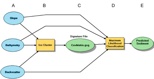
The detailed methods used for the Quantitative Bottom Classification of the nearshore area are presented in this appendix.  The classification was carried out within ArcGIS Modelbuilder ver. 9.2.  The map of predicted sediment type in figure 4.8 (panel D) was produced by using three steps: exploration, cluster analysis, and maximum likelihood classification.  The classification was limited to the nearshore area, where we have high-quality bathymetric data from interferometric sonar and backscatter data from towed sidescan sonar.

1. Exploration

First, the relationship between backscatter value and grain size was examined for meaningful division in class breaks.  Mean backscatter values, expressed as digital numbers (DN), were extracted from the sidescan-sonar mosaic at 14 sampling locations and plotted against mean grain size (fig. 4.7).  The DN values were obtained from a circle with a 5-m radius that was centered on each sampling location to account for navigational uncertainty.  The mean grain size of these samples fell in two distinct classes that are described by the Wentworth scale (Wentworth 1922) for sediment texture: fine to very fine sand (3.4 to 2.1 phi) and coarse sand (0.7 to 0.0 phi).  Because no samples of medium sand were collected, the two classes were clearly separated.  On the basis of the bimodal distribution of grain size, the entire nearshore seafloor was divided into these two general classes of sediment (i.e., very fine to fine sand and coarse sand).

2. Cluster Analysis

The two grain-size classes from the sediment samples in step 1 served as input to an iterative self-organizing (ISO) clustering function used to classify the three input rasters (fig A4.1). The ISO cluster algorithm calculated the covariance values between the overlapping cells in each of the three input layers (fig A4.1a) to produce a signature file (fig A4.1c). The input layers for the analysis were 5-m resolution bathymetry (depth), backscatter, and slope (degrees). The backscatter data, originally processed to 1-m resolution, were aggregated to 5-m resolution to match the resolution of the bathymetry and slope.

Figure A4.1. ArcGIS Modelbuilder flow diagram showing the three input raster layers (A).  The ISO clustering function in (B) produces the signature file (C).  The Maximum Likelihood Classification (D) is then used, along with the signature file and the three raster layers, to produce the final grid of predicted sediment type (E). Click on figure for larger image.

3. Maximum Likelihood Classification

The signature file from step 2 was input to a Maximum Likelihood Classification (MLC) (fig A4.1d) routine along with the three original rasters to produce an 8-bit unsigned integer raster (fig A4.1e).  Each cell of this raster is assigned an integer value of 1 through 3 based on the maximum likelihood that the cell falls into one of the user-defined classes.  Although the intent was to classify the bottom in two different classes, the guiding rule for this method is to use at least the same number of classes (3) as input layers (3) and then aggregate similar classes (Jensen, 2005).  Based on this principle, classes 2 and 3 were combined into class 2.  The symbology of the output raster is edited to facilitate cartographic presentation and illustration (Panel D, fig. 4.8).