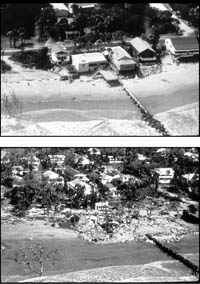
Figure 1.1.  Photographs of the beach at Folly Island taken before (top) and after (bottom) Hurricane Hugo struck the coast of South Carolina in October 1989 (published by permission of the National Oceanic and Atmospheric Administration Photo Library accessed online July 1, 2007 at http://www.photolib.noaa.gov). [larger version]

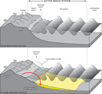Figure 1.2.  Schematic diagrams of the active beach system, which extends from the dunes to the inner edge of the continental shelf.   TOP: During fair weather, sediment is stored in the upper beach and dunes.  The relatively broad, flat berm is dry at high tide.  The intertidal beach is relatively narrow, and the seaward-sloping shoreface forms a concave-upward surface beneath the waves.  BOTTOM: During stormy weather, waves and currents erode the berm and dunes.   Sediment is transported offshore into deeper water (red arrow) and produces a broader, more gently sloping intertidal beach and shoreface.  Sediment temporarily stored offshore typically moves back onto the beach in the weeks and months following a storm. [larger version]

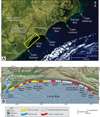Figure 1.3.  (A) Satellite image showing the location of the Grand Strand study area on the North and South Carolina coasts (published by permission of the National Aeronautics and Space Administration–Visible Earth program accessed July 1, 2007 online at http://visibleearth.nasa.gov/). (B) Map showing physiographic and geographic features on the Grand Strand.  Types of coastal landforms are indicated by the color-coded bands parallel to the coast. [larger version]

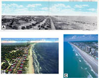Figure 1.4.  Views of the Grand Strand before and after high-density oceanfront development.  (A) Picture postcard of Myrtle Beach Pavilion area with boardwalk and small structures behind a natural dune.  Photograph taken by W. C. Johnson around 1927 (published by permission of the Lake County (IL) Discovery Museum, Curt Teich Postcard Archives).  (B) Picture postcard of the Crescent Beach and Ocean Drive Beach sections of North Myrtle Beach around 1955 (published by permission of the South Caroliniana Library, University of South Carolina–Columbia).  During this period, single-family cottages represented most of the development and, although structures did stand close to the shoreline, the integrity of primary coastal dunes was preserved.  (C) Photograph of oceanfront along the downtown section of Myrtle Beach around 2000 (published by permission of the Myrtle Beach Area Convention and Visitors Bureau). High-rise condominiums and hotels now dominate development along the Grand Strand.  In many areas, structures stand directly adjacent to the beach and frontal dunes are absent. [larger version]

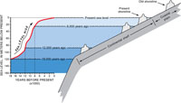Figure 1.5.  Diagram showing typical response of shorelines to rising sea level.  When sea level rises, the ocean advances over the land and shorelines retreat or move landward.  The red line shows the irregular rate of sea level rise since the end of the last Ice Age (adapted from Fairbanks, 1989).  At that time, sea level was about 120 m below present and the shoreline was located at or near the edge of the continental shelf.  The steep section of the red line between 12,000 and 8,000 years ago shows a rapid rise in sea level that caused shorelines to migrate landward at a faster rate.  Even small increases in sea level can cause shorelines to retreat large distances across the gently sloping continental shelf and coastal plain.  The rate of sea-level rise slowed about 6000 years ago, thereby allowing shorelines to stabilize near their present location.  Old shoreline deposits on the coastal plain (see Figure 1.6) were formed at least 125,000 years ago when sea level was higher than today. [larger version]

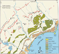Figure 1.6.  Map showing ancient barrier islands and other shoreline features on the coastal plain of the Long Bay region (modified from DuBar and others, 1974).  The shorelines formed at former highstands of sea level that flooded the coastal plain multiple times over the last 3-4 million years. The relict shorelines step down in elevation and become progressively younger toward the modern coast, with the highest and oldest (Orangeburg Scarp) farthest inland.  All have been heavily dissected by rivers and streams. [larger version]

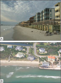Figure 1.7. Photographs showing impact of engineering structures on South Carolina's beaches.  (A) Seawall at Garden City Beach in February 2007.  Seawalls are constructed to protect structures from being undermined as the shoreline migrates landward. This image highlights the dilemma between saving structures and maintaining a usable beach (published by permission of M. Scott Harris, College of Charleston, Charleston, South Carolina). (B) Southern end of the seawall at the Debordieu community in June, 2005.  The adjacent unarmored section of coast is left free to migrate, leaving the seawall-protected property in a precarious position seaward of the natural shoreline.  Beach nourishment has been used at this site to prevent failure of the seawall and temporarily provide some beach function (published by permission of Paul Gayes, Coastal Carolina University, Conway, South Carolina). [larger version]

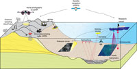Figure 2.1. Schematic diagram showing the different techniques used to investigate the active beach system along the Grand Strand.  Acoustic instruments (sidescan sonar, swath bathymetry and subbottom profilers) provide information on the distribution of sediments, topography, and underlying structure of the shallow seafloor adjacent to the beach.  On land, ground-penetrating radar (GPR) determines the thickness and structure of sediment beneath the beach and dunes. Sediment grain size, composition, and age are determined by direct sampling of offshore and onshore deposits.  To monitor short-term changes in beach morphology, precise elevation measurements are collected from the dune to the edge of the inner shelf by using all-terrain vehicles on land and small boats offshore as part of the Beach Erosion Research and Monitoring (BERM) program.  Aerial photography and Light Detection and Ranging (LIDAR) are used to survey and quantify changes along the coast.  Differential Global Positioning Systems (DGPSs) are used to locate all data accurately. [larger version]

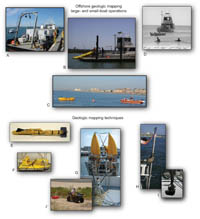Figure 2.2A.  Mapping operations of the South Carolina Coastal Erosion Study (SCCES): (A) Research vessel at dock preparing for departure; (B) Small research vessel at dock with subbottom profiler towed from the stern; (C) Subbottom profiler towed by rigid-hull inflatable boat directly off the beach; (D) Subbottom profiler towed in very shallow water away from the beach; (E) Sidescan-sonar system; (F) Subbottom profiler; (G) Subbottom profiler deployed off the stern of small coastal research vessel; (H) Swath bathymetric system configured as a side-mount; (I) Swath bathymetric transducer deployed off the bow of a small vessel; and (J) All-terrain vehicle (ATV) towing a ground-penetrating radar (GPR) sled across the beach. [larger version]

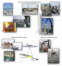Figure 2.2B. Mapping operations of the SCCES (continued): (A) Collection of sediment core on the beach; (B) Large coring rig for deep sampling; (C) Video camera used to collect images of the seafloor; (D1) Grab sampler used to collect sediment from the seafloor; (D2) Sediment samples stored in bags for laboratory analysis; (E1) Photograph of a sediment core; (E2) Collection of offshore sediment with vibracores; (F1) Rigid-hull inflatable boat measuring beach profiles in nearshore area; (F2) ATV measuring beach profiles onshore; (G) Aerial photograph used in shoreline-change analysis of North Myrtle Beach; (H) LIDAR systems rapidly map topography over extensive areas of coast; (I) and (J) Deployment of oceanographic instruments on a tripod (rigid three-leg structure) that will be anchored to the seafloor. [larger version]

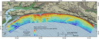Figure 2.3.  Map showing bathymetry offshore of the Grand Strand. Water depths in survey area range from 2 to 14 m. [larger version]

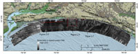Figure 2.4. showing acoustic backscatter intensity, as measured with sidescan sonar, on the shallow seafloor of Long Bay.  Backscatter intensity is a measure of the hardness and roughness of the seafloor.  In general, higher values (light tones) represent rock, coarse sand, and gravel.  Lower values (dark tones) generally represent fine sand and muddy sediment. Backscatter values are represented as digital numbers assigned to the pixels within the imagery, ranging from 0 (black) to 255 (white). Backscatter data are combined with laboratory analysis of sediment samples to interpret the surficial geology of the seafloor.  Locations for Figures 2.5, 2.6, and 2.7 are displayed. [larger version]

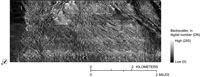Figure 2.5.  Enlarged section of the sidescan-sonar image in Figure 2.4 shows the complexities of the shallow seafloor offshore of Myrtle Beach.  Intricate patterns of high backscatter (light tones) and low backscatter (dark tones) represent exposures of rock and fine sand deposits, respectively.  Backscatter values are represented as digital numbers assigned to the pixels within the imagery, ranging from 0 (black) to 255 (white).  See Figure 2.4 for location. [larger version]

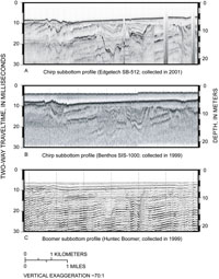Figure 2.6.  Subbottom profiles collected with three different systems along the same trackline offshore of Murrells Inlet.  A constant seismic velocity of 1.5 km/s was used to convert traveltime to depth.  Modified from Baldwin and others (2004). ~, about. [larger version]

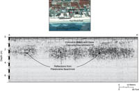Figure 2.7.  TOP: Aerial photograph of Myrtle Beach showing location of ground-penetrating radar (GPR) profile collected at Hurl Rock Park.  BOTTOM: GPR profile showing Pleistocene beachrock buried 1–2 m beneath the beach.  These rocks are episodically exposed when storms erode the beach (see photograph in Figure 4.4B). [larger version]

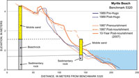Figure 2.8. Beach profiles collected at Myrtle Beach over a 10-year period showing changes in beach shape.  Blue lines represent the beach before and after Hurricane Hugo struck in 1989, causing extensive erosion.  The 1997 pre-nourishment profile shows limited amounts of mobile sediment overlying beachrock and sedimentary rock, which commonly were exposed along the beach and shoreface.  Later that year, a large amount of new sediment was pumped onto the beach and buried the rocky outcrops beneath a wide, sandy berm.  Ten years after the nourishment, the beach fill has eroded but continues to cover the rocks.  See Figure 4.5 for location. [larger version]

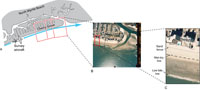Figure 2.9. A) Schematic showing the flight path of an aerial photographic survey that follows the coastline in North Myrtle Beach.  Surveys are conducted at low tide with adjacent, overlapping photographs to allow for continuous coverage. B) Example of aerial photograph showing coastal development and shoreline morphology at Cherry Grove.  C) Enlarged area of the photograph showing prominent features such as the sand fence, wet-dry line and low-tide line.  The wet-dry line is typically used to delineate shoreline position on aerial photographs.  Shorelines delineated from successive surveys are compared to assess change in position over time. [larger version]

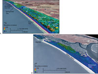Figure 2.10. Aerial photographs overlain with Light Detection and Ranging (LIDAR) topography show A) dense coastal development at Myrtle Beach, and B) undeveloped beach and dunes at Waites Island.  Data were collected in 2006 as part of the National Coastal Mapping Program by the U.S. Army Corps of Engineers.  Frequent surveys allow geologists to assess short-term change to the shoreline, such as the immediate impact of large storms. [larger version]

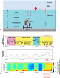Figure 2.11. A) Schematic diagram showing oceanographic instruments deployed offshore of Myrtle Beach as part of the South Carolina Coastal Erosion Study (SCCES).  The tripod frame and instruments were anchored to the seafloor, collecting data at regular intervals over a six-month period. ADCP, Acoustic Doppler current profiler.  Modified from Bothner and Butman (2007).  B) Graphs showing data for wind speed and direction (top), wave height (center), and suspended sediment concentrations in the water column (bottom).  Red box indicates a period of strong winds and high waves on February 26-27, 2004, which mobilized abundant sediment from the seafloor and suspended it in the water column. [larger version]

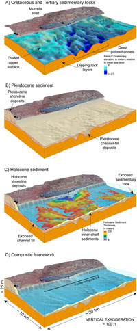Figure 3.1. Schematic diagrams of the Murrells Inlet area showing the primary components of the Grand Strand geologic framework, from the deepest and oldest to the shallowest and youngest.  See Figure 3.2 for the location of this area.  A) Layered units of tilted Cretaceous and Tertiary sedimentary rocks underlie the entire coastal system.  Relief on the surface of the rocks shows large channels deeply incised by rivers and streams at times of lower sea level.  Elevations are shown relative to mean sea level (MSL).   B) Pleistocene channel fills are regionally truncated by a low-relief erosional unconformity.  Pleistocene shoreline deposits form the core of the coastal upland.  C) Holocene shoreline and inner-shelf sediments overlie the regionally extensive erosional unconformity.  Wedge-shaped shoreline deposits lie above and adjacent to the eroded remains of older Pleistocene shoreline deposits, and thin considerably across the shoreface onto the inner shelf.  Rocks and channel fills are exposed at the seafloor over extensive areas lacking Holocene sediment cover.  Deposits up to 6 m (20 ft) thick are primarily associated with tidal inlets.  D) A composite view of the framework beneath the coastline and seafloor.  Black line indicates the location of the seismic-reflection profile in Figure 3.4.  Red lines in diagrams A-C indicate erosional unconformities.  The onshore land image was compiled from 1999 digital-orthophoto quarter-quadrangles provided by the South Carolina Department of Natural Resources. <, deeper than; ~, about. [larger version]

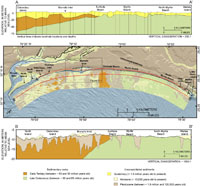Figure 3.2. Surficial geologic map (middle) and geologic cross sections (top and bottom) showing the regional geologic framework of the Grand Strand coast and Long Bay inner shelf.  The underlying foundation is composed of Cretaceous and Tertiary sedimentary rocks, which are incised by deep channels of the ancestral Pee Dee River.  On the inner shelf (section B-B'), sedimentary rocks and Pleistocene channel-fills are regionally truncated by a low-relief erosional unconformity and overlain by a thin, patchy layer of unconsolidated Holocene sediment.  Landward of the shoreline (section A-A'), channel-fill deposits are overlain by a section of Quaternary shoreline units between about 10 and 30 m (33-100 ft) thick.  Onshore geology is generalized from McCarten and others (1984) and Owens (1989).  Offshore geology is from Baldwin and others (2007).  Cross section A-A' is modified from Putney and others (2004), and B-B' is from interpretation of seismic reflection-profiles.  The background shaded-relief imagery was constructed by using the NOAA-NGDC coastal-relief model. ~, about. [larger version]

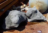Figure 3.3. Photograph of Late Cretaceous sedimentary rock excavated during engineering work offshore of northern Myrtle Beach (published by permission of James Daigle, Sunland Construction Inc., Eunice, Louisiana). [larger version]

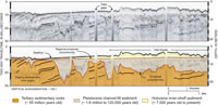Figure 3.4. Seismic-reflection profile offshore of the Murrells Inlet area.  TOP: Original data showing vertical slice through the upper 20 m (66 ft) of the seafloor.  BOTTOM: Interpreted profile showing the primary framework components underlying the inner shelf.  Location indicated in Figure 3.1D.  Two-way traveltime is in milliseconds and depth is in meters.  A constant seismic velocity of 1.5 km/s was used to convert from two-way traveltime to depth (modified from Baldwin and others, 2006). ~, about; <, less than. [larger version]

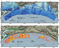Figure 3.5. A) Map showing topography on top of Cretaceous and Tertiary sedimentary rocks (base of Quaternary elevation) beneath the Grand Strand.  Elongate depressions (shown in the darkest blue colors) crossing this generally low-relief surface represent paleochannels incised by fluvial systems since the Late Pliocene (about 2.1 million years ago).  The largest paleochannels were produced by the Pee Dee River, which has occupied multiple courses across the region during the geologic past (see Figure 3.9).  Modified from Putney and others (2004) and Baldwin and others (2007). >, higher than; <, deeper than.  B) Map showing thickness of Holocene inner-shelf sediments, which generally increase in abundance from north to south. Over large areas Holocene sediments are less than 0.5 m (1.6 m) thick or absent.  The largest accumulations (up to 6 m or 20 ft thick) generally form shoal complexes that extend seaward from tidal inlets.  A notable exception is a north-south oriented, shore-oblique shoal offshore of Myrtle Beach.  Modified from Baldwin and others (2007).   The background shaded-relief imagery was constructed by using the NOAA-NGDC coastal relief model and USGS hydrography data. [larger version]

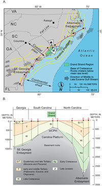Figure 3.6. A) Map showing major structure and physiography of the southeast U.S. continental margin.  Yellow contour lines indicate depth to the base of Cretaceous sedimentary rocks (adapted from Horton and others, 1991).  Seaward-bulging contours indicate relatively thin post-Cretaceous deposits across the Carolina Platform, a major structural high that underlies the coastal plain and continental shelf.  The Grand Strand is located near the apex of the Mid-Carolina Platform High (MCPH), which is the shallowest, most stable portion of the Carolina Platform.  Gray arrows indicate the direction of an ancient ocean current, much like the modern Gulf Stream, which flowed across the MCPH during the Middle to Late Eocene and caused prolonged nondeposition and erosion (generalized from Popenoe, 1985).  B) Geologic cross section constructed from deep borehole data (black dots #1-9) along the coast (red line in part A).  Cretaceous rocks are at or near the surface along the Grand Strand, but more deeply buried by younger deposits within the Albemarle and Southeast Georgia Embayments, structural lows that bound the Carolina Platform on either side.  Figure adapted from Gohn (1988). [larger version]

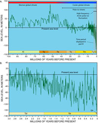Figure 3.7. A) Global sea level and general climate conditions over the past 100 million years.  Grey box indicates ongoing period of high-frequency sea-level changes due to ice-volume fluctuations over the past 3 million years. B) Section showing sea level over the last 3 million years enlarged from the graph in part A. Sea-level curves simplified from Miller and others (2005); climate and glacial ice-information generalized from Moran and others (2006).  Color coded bars along the bottom of each part indicate geologic time: Kl = Late Cretaceous, Tp = Paleocene, Te = Eocene, To = Oligocene, Tm = Miocene, Tpl = Pliocene, Q = Quaternary, Qp = Pleistocene, and Qh = Holocene. [larger version]

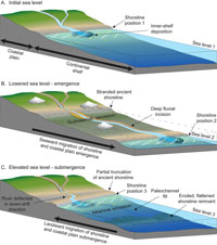Figure 3.8. A three-phase conceptual model showing evolution of the Grand Strand region over a cycle of emergence-submergence driven by relative sea-level changes.  Schematic diagrams illustrate shoreline migration seaward and landward across the coastal plain and continental shelf.  A) Initial sea level is high; stable shoreline deposits develop at relatively high elevation. B) Sea level falls and shoreline migrates seaward.  Inner shelf emerges, leaving older shoreline stranded high on the coastal plain.  Unconformity produced by broad subaerial erosion and deep fluvial incision.  C) Sea level rises and shoreline migrates landward.  Eroded remnants of lowstand shoreline stranded on the continental shelf.  Erosion by waves and currents generally flattens the landscape and partially truncates older highstand shoreline.  As sea level stabilizes, shoreline deposits accumulate at higher elevations and cause river mouth to migrate downdrift. [larger version]

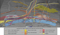Figure 3.9.  Perspective view of the Grand Strand region looking towards the northwest.  Arrows indicate changing locations of the Pee Dee River over time (generalized from Baldwin and others, 2006).  Progressive, southwestward deposition along ancient shorelines gradually deflected the river toward the southwest.  Older (more landward) shorelines initially trended east-west, but rotated to northeast-southwest as they were deposited progressively closer to the modern coastline.  Shaded relief of the regional surface defining the base of Quaternary sediments (also displayed in Figure 3.5a) shows that the river carved at least seven distinct courses across the region prior to its current configuration, which flows through Winyah Bay.  The background-shaded relief imagery was constructed by using the NOAA-NGDC coastal-relief model. >, higher than; <, deeper than. [larger version]

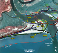Figure 4.1.  Aerial photograph showing historical shorelines from 1856 to 1983 around Waites Island and Little River Inlet.  Shore-normal transects (gray lines) starting at a baseline 500 m offshore (red line) and extending inland for 2000 m, were drawn every 25 m along the coast.  Where a transect intersected a former shoreline position (colored dots), the distance from the baseline was used to calculate the average rate of shoreline change over that time period.  See Figure 4.2 for location. [larger version]

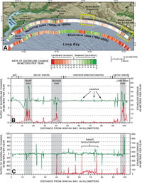Figure 4.2. (A) Map view of the Grand Strand showing rates of shoreline change as color-coded bands parallel to the coast.  Historical rates are based on shoreline positions derived from maps, charts, and air photographs.  Short-term rates are based on shoreline positions measured by LIDAR surveys.  Rates are calculated by using the linear rate-of-regression method (Thieler and others, 2003), which runs a best-fit line through all available data points.  (B) Graph showing historical rates of shoreline change (green line) from the 1850s to 1980s.  Highest rates of change are in the vicinity of inlets; lowest rates are along mainland-attached beaches.  Standard error (red line) of the measurements indicates variability in shoreline positions through time.  If the shoreline at a particular area shows high variability (that is, it moves back and forth a lot), standard error is high.  Shoreline positions along inlets and barrier islands have higher variability and lower variability along mainland-attached beaches.  (C) Graph showing short-term rates of shoreline change between 1996 and 2000.  Shoreline positions along smaller inlets, swashes, and the beach renourishment project at Myrtle Beach show the largest amount of variation at this time scale. [larger version]

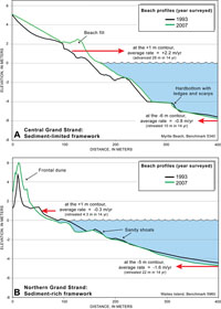Figure 4.3. (A) Typical profile at Myrtle Beach is relatively steep and interrupted by rocky ledges and scarps.  This area was nourished in 1998, and a small wedge of beach fill remains visible in the 2007 profile. (B) Typical profile at Waites Island is relatively gently sloping due to abundant sand associated with inlet shoals.  The profile has steepened in both locations due to continued erosion and landward migration (that is, retreat) of the mid- to lower shoreface (red arrows). See Figures 4.5 and 4.6 for locations of the profiles. [larger version]

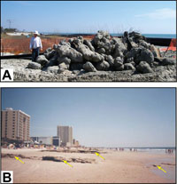Figure 4.4.  (A) Large boulders excavated during construction of storm water outfall near 52nd Ave. North, Myrtle Beach (published by permission of James Daigle, Sunland Construction Inc., Eunice, Louisiana).  The boulders came from rocky deposits that lie at shallow depths beneath Grand Strand beaches.  (B) Rocks indicated by arrows exposed by beach erosion at Hurl Rocks Park, Myrtle Beach (published by permission of Paul Gayes, Coastal Carolina University, Conway, South Carolina.)  Sediment removed by storms typically returns in times of fair weather and rebuilds the beach. [larger version]

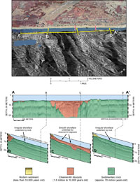Figure 4.5.  Shoreface geology along the central Grand Strand at Myrtle Beach.  (TOP) Perspective view showing a complex pattern of acoustic backscatter on the shallow seafloor.  High backscatter (light shades) generally indicates coarse sand, gravel, and rock.  Low backscatter (darker shades) generally indicates sandy or muddy sediment.  (A-D) Interpreted subbottom profiles showing the geologic framework underlying the shoreface. ~, about.  See Figure 4.2 for location. [larger version]

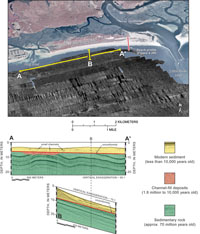Figure 4.6.  Shoreface geology along the northern Grand Strand at Waites Island.  (TOP) Perspective view showing a complex pattern of acoustic backscatter on the shallow seafloor.  High backscatter (light shades) generally indicates coarse sand, gravel, and rock.  Low backscatter (darker shades) generally indicates sandy or muddy sediment.  (A-B) Interpreted subbottom profiles showing the geologic framework underlying the shoreface. ~, about.  See Figure 4.2 for location. [larger version]

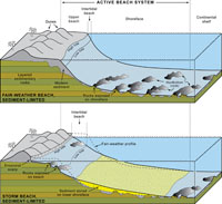Figure 4.7.  Schematic diagrams showing seasonal changes in a sediment-limited beach typical of the central Grand Strand.  Vertical scale is highly exaggerated to emphasize subtle topographic features.  (TOP) During times of fair weather, sediment is transported landward from the shoreface and stored in the dunes and berm.  Upper surface of erosion-resistant sedimentary rock is exposed in shallow-water areas adjacent to the beach.  (BOTTOM) During times of stormy weather, the beach is eroded and sedimentary rock is locally exposed on the broad intertidal beach.  The eroded sediment is transported offshore, where it buries rocky areas and produces a relatively smooth, sandy shoreface. [larger version]

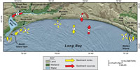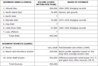
Figure 5.1.  Diagram showing the components of a conceptual long-term sediment budget for the Grand Strand region (modified from Gayes and others, 2003).  Numbered arrows indicate the general direction of sediment movement.  Sediment sinks include: 1. Winyah Bay, 2. North Island Spit, 3. North Inlet, 4. Murrells Inlet, 5. Hogg Inlet, 6. Little River Inlet, and 7. loss offshore.  Sediment sources include: 8. rivers, 9. beach and shoreface erosion, and 10. inner-shelf erosion.  See Table 5.1 for estimates of sediment volumes associated with each component. [larger version]

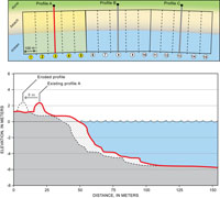Figure 5.2.  Diagrams showing how volumes were calculated for sediment eroded from beach and shoreface deposits.  (TOP) Plan view of a beach divided into 15 equal segments, each measuring 100 m wide and extending from the dune crest to the shoreface.  An existing beach profile (A, B, or C) is assigned to nearby segments of beach.  In this example, profile A (red line) represents segments 1–5.  Profiles B and C represent segments 6–10 and 11–15, respectively.  (BOTTOM) The existing profile is moved landward based on the long-term erosion rate that has been established for each beach segment (see Figure 4.2).  Profile shape remains constant, and the area between the eroded profile and the existing profile represents the sediment released in one year.  For example, if the beach in segment 1 is eroding rapidly at 8 m/yr (26 ft/yr), profile A is translated 8 m (26 ft) landward of its original position, and the region between the two profiles (diagonal line pattern) represents the annual volume of eroded sediment.  Values are added for all segments to determine the total amount of new sediment that is contributed to the regional sediment budget. [larger version]

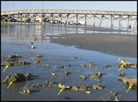Figure 5.3.  Photograph showing pieces of sedimentary rock (arrows) on Surfside Beach after a 1999 storm.  The corals attached to these rock fragments typically live more than 1 km (0.6 mi) offshore of the beach (from Gayes and others, 2003). [larger version]

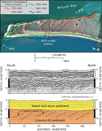Figure 5.4.  TOP: Aerial photograph of the North Island spit at the southern end of the Grand Strand, showing the positions of five historical shorelines.  Prominent beach ridges (dashed lines) that predate the historical record were produced as the spit grew from north to south.   BOTTOM: Ground-penetrating radar profile showing the internal structure of the spit, which consists of sandy sediment over 10 m thick.  Steeply dipping layers in the lower unit (orange) formed as sediment, carried by south-directed longshore currents, filled the channel at the entrance to Winyah Bay.  Beaches and dunes later developed on top of the channel-fill sediment, producing an upper deposit of fine sand (yellow) that exhibits wavy, nearly flat-lying layers.  The calculation of sediment volume stored in the spit from 1872–1983 (see Table 5.1) is based on the prograding upper unit and underlying channel fill. ~, about. [larger version]

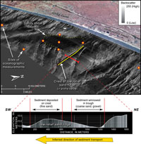Figure 5.5. (TOP) Perspective view of the inner shelf offshore of Myrtle Beach showing sidescan-sonar imagery draped over bathymetry.  High backscatter values (light tones) generally represent rock, gravel or coarse sand.  Low backscatter values (dark tones) generally represent fine sand or muddy sediment.  Oceanographic instruments were deployed at eight sites (red circles) on and near a large sandy shoal to determine the physical processes that control sediment transport around the feature.  (BOTTOM) Bathymetric profile across a low-relief sand ridge.  The steeper slope faces toward the southwest, indicating the direction of net sediment transport.  Finer sediment has been winnowed from the trough and northeast-facing side of the ridge, leaving a lag of coarse sand and gravel.  Fine sand has been deposited on the crest and southwest-facing side.  Modified from Denny and others (2006). [larger version]

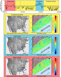Figure 5.6.  Measurements of wind speed and direction (top) collected offshore of Myrtle Beach from February 8–29, 2004.  Additional data for this time period are shown in Figure 2.11B.  Weather maps in bottom panels show three different storm patterns crossing the region.  Simulation results for each storm show the general direction of sediment transport (arrows) and predicted areas of sediment erosion and deposition on the inner shelf (colors).  The 8m bathymetric contour is displayed in red within the simulation results.  See main text for description of storms and predicted movement of shelf sediment. [larger version]

Table 3.1. Geologic time scale from the Jurassic Period to the present day.  Stippled patterns indicate long segments of geologic time not represented by deposits in the Grand Strand region (that is, times of erosion or nondeposition). Simplified from Geological Society of America (1999). [larger version]

Table 3.2. Table describing three general scales of influence on the geologic evolution of the Grand Strand. [larger version]

Table 5.1.  A conceptual sediment budget for the Grand Strand region.  Table lists estimated volumes of mobile sediment annually lost to sinks and gained from different sources (modified from Gayes and others, 2003).  Numbers in first column correspond to numbered arrows in Figure 5.1.  Dredging records are from C. Mack (U.S. Army Corps of Engineers, oral communication, 2003). [larger version]