 |
Figure 1. Index map of the coastal waters off southeastern New England showing location of the H11922 study area west of Martha's Vineyard, Massachusetts (red polygon). Also shown are (1) the locations of earlier studies off Massachusetts including the Outer Cape Survey (Poppe and others, 2006) and National Oceanic and Atmospheric Administration surveys H11076 – Quicks Hole (Poppe and others, 2007a), H11079 – Great Round Shoal Channel (Poppe and others, 2007b), H11077 – Woods Hole (Poppe and others, 2008), H11346 – Edgartown (Poppe and others 2010); (2) earlier studies off Rhode Island including H11320 (McMullen and others, 2007), H11321 (McMullen and others, 2008), H11322 (McMullen and others, 2009a), and H11996 (McMullen and others, 2011); and (3) the extent of digitally reprocessed seismic-reflection data (McMullen and others, 2009b) completed as part of this series (gray polygons). |
 |
Figure 2. Map, modified from Stone and Borns (1986) and Gustavson and Boothroyd (1987), showing locations of end moraines (black polygons) in southern New England and on Long Island, New York. The Ronkonkoma-Nantucket moraine marks the Laurentide Ice Sheet's southern extent at glacial maximum about 20-24 ka and the Harbor Hill-Roanoke Point-Charlestown-Buzzards Bay moraine represents ice sheet position after a readvance around 18 ka (Uchupi and others, 1996). Underwater extensions of the moraines are shown as dashed lines. Study area is shown as a red polygon. |
 |
Figure 3. Segment of Uniboom seismic-reflection profile collected along the east-west axis of the study area (RV Asterias 75-6, line 11; O'Hara and Oldale, 1980; McMullen and others, 2009b). Profile reveals a stratigraphic section composed of coastal plain, glacial drift, estuarine and transitional, and marine deposits. Location of seismic profile is shown in figure 21. |
 |
Figure 4. Segment of Uniboom seismic-reflection profile collected across a bathymetric high in the eastern part of the study area (RV Asterias 75-6, line 31; O'Hara and Oldale, 1980; McMullen and others, 2009b). The high is cored by coastal plain sediments and mantled by glacial till, as evidenced by the presence of boulders on the sea floor. Location of seismic profile is shown in figure 21. |
 |
Figure 5. Photograph of the Gay Head cliffs on Martha's Vineyard, Massachusetts. The colorful cliffs are composed of dislocated and thrust-faulted coastal plain deposits, capped by a veneer of glacial till. |
 |
Figure 6. Port-side view of the National Oceanic and Atmospheric Administration Ship Thomas Jefferson at sea. Note that the 30-foot survey launch normally stowed on this side of the ship has been deployed. |
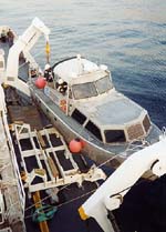 |
Figure 7. Image showing launch 3102 being deployed from the National Oceanic and Atmospheric Administration Ship Thomas Jefferson. |
 |
Figure 8. Starboard-side view of the National Oceanic and Atmospheric Administration launch 3102 at sea. |
 |
Figure 9. The RESON SeaBat 8101 multibeam echosounder hull-mounted to the National Oceanic and Atmospheric Administration launch 3102. |
 |
Figure 10. The RESON Seabat 8125 multibeam echosounder hull-mounted to National Oceanic and Atmospheric Administration launch 3101. |
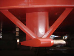 |
Figure 11. The RESON 7125 multibeam echosounder hull-mounted to the National Oceanographic and Atmospheric Administration Ship Thomas Jefferson. |
 |
Figure 12. Brooke Ocean Technology Moving Vessel Profiler with a Sea-Bird Electronics, Inc., conductivity-temperature-depth (CTD) profiler used to correct sound velocities for the multibeam data. |
 |
Figure 13. Sea-Bird Electronics, Inc., SEACAT conductivity-temperature-depth (CTD) profiler. Data derived from frequent deployments of this device were used to correct sound velocities for multibeam data collected aboard the launches. |
 |
Figure 14. Image shows a port-side view of the U.S. Geological Survey (USGS) RV Rafael that was used to collect bottom photography and sediment samples during USGS cruise 2010-033-FA. |
 |
Figure 15. Image shows a starboard-side view of the RV Connecticut that was used to collect bottom photography and sediment samples during U.S. Geological Survey cruise 2010-005-FA. |
 |
Figure 16. View of the small SEABOSS, a modified Van Veen grab equipped with still and video photographic systems, mounted on the aft starboard side of the RV Rafael. Note the winch mounted on the davit (left) and the take-up reel for the video-signal and power cable (right). |
 |
Figure 17. Map showing the station locations used to verify the acoustic data with bottom sampling and photography during U.S. Geological Survey cruises 2010-033-FA and 2010-005-FA. |
 |
Figure 18. Correlation chart showing the relationships between phi sizes, millimeter diameters, size classifications (Wentworth, 1922), and ASTM and Tyler sieve sizes. Chart also shows the corresponding intermediate diameters, grains per milligram, settling velocities, and threshold velocities for traction. |
 |
Figure 19. Sediment classification scheme from Shepard (1954), as modified by Schlee (1973). |
 |
Figure 20. Digital terrain model (DTM) of the sea floor produced from multibeam bathymetry collected during National Oceanic and Atmospheric Administration survey H11922 west of Gay Head, Massachusetts, in eastern Rhode Island Sound. Image is sun-illuminated from the north and vertically exaggerated 5x. Hotter colors are shallower areas; cooler colors are deeper areas. See key for depth ranges. |
 |
Figure 21. Locations of detailed planar views of the digital terrain model (yellow polygons), Uniboom seismic-reflection profiles shown in figures 3 and 4 (green lines), and depth profiles of bedform morphology (red dots) shown in figure 27. |
 |
Figure 22. Detailed planar view of the bathymetric data collected during National Oceanic and Atmospheric Administration survey H11922 showing the extent of the scour on the bathymetric high in the northeastern part of the study area and the locations of stations 922-1, 922-2, 922-3, and 922-194. Note the presence of boulders on the floor of the scour depression and the field of megaripples on the adjacent seabed. Location of view is shown in figure 21. |
 |
Figure 23. Detailed planar view of the bathymetric data collected during National Oceanic and Atmospheric Administration survey H11922 showing the extent of the scour in the southeastern part of the study area and the locations of stations 922-7 and 922-8. Note the flat, featureless appearance of the surrounding seabed composed of Holocene marine sediments. Location of view is shown in figure 21. |
 |
Figure 24. Detailed planar view of the bathymetric data collected during National Oceanic and Atmospheric Administration survey H11922 showing the gradual transition from winnowed bouldery sea floor to the surrounding Holocene deposits in the south-central part of the study area and the location of station 922-14. Note the presence of megaripples, and fingers of eroded Holocene deposits creating a valley and ridge type topography. Location of view is shown in figure 21. |
 |
Figure 25. Detailed planar view of the bathymetric data collected during National Oceanic and Atmospheric Administration survey H11922 showing the complex pattern of scour in the northwestern part of the study area and the locations of stations 922-18, 922-20, and 922-22. Note the presence of erosional outliers. Location of view is shown in figure 21. |
 |
Figure 26. Detailed planar view of the bathymetric data collected during National Oceanic and Atmospheric Administration survey H11922 showing small rocky outcrops in the north-central part of the study area. Note that the minor scour present around some of the outcrops is symmetrical. Location of view is shown in figure 21. |
 |
Figure 27. Cross-sectional views of megaripples from the digital terrain model produced from bathymetric data collected during National Oceanic and Atmospheric Administration survey H11922. Bedform asymmetry and slip-face orientation (Reineck and Singh, 1980) indicates net northwestward and northeastward sediment transport in profiles A and B, respectively. The megaripples in profile C are predominantly symmetrical. Locations of profiles are shown in figure 21. |
 |
Figure 28. Map showing the station locations from U.S. Geological Survey cruises 2010-033-FA and 2010-005-FA, that were used to verify the acoustic data, color coded for sediment texture. Hotter colors are coarser grained sediment; cooler colors are finer grained sediments. |
 |
Figure 29. Distribution of sedimentary environments based on the digital terrain model from National Oceanic and Atmospheric Administration survey H11922 and the sampling and photography data from U.S. Geological Survey cruises 2010-033-FA and 2010-005-FA that were used to verify the acoustic data. Areas characterized by processes associated with erosion or nondeposition, coarse bedload transport, and sorting and reworking are shown. |
 |
Figure 30. Bottom photographs from stations 922-3 and 922-7 showing the sessile fauna and flora that commonly cover boulders in the high-energy environments. Station locations are shown in figures 17, 22, 23, and 28. |
 |
Figure 31. Bottom photographs from stations 922-13 and 922-14 showing a view of the gravel sea floor that surrounds the bouldery sea floor in the south-central part of the study area. Note the presence of a thin veneer of mud on the gravel. Station locations are shown in figures 17 and 28. |
 |
Figure 32. Bottom photographs from stations 922-10 and 922-16 showing views of the rippled sea floor composed of fine-grained sand. Note the presence of burrows, worm tubes, and amphipod tubes in the ripple troughs. Station locations are shown in figures 17 and 28. |
 |
Figure 33. Bottom photographs from stations 922-12 and 922-17 showing a view of the flat to undulating to faintly rippled sea floor composed of muddy sand typical of the deeper parts of the study area. Note the presence of shrimp burrows and worm tubes. Station locations are shown in figures 17 and 28. |
 |
Figure 34. Bottom photographs showing a comparison of the undulating muddy sand at station 922-22, typical of the Holocene sediments in Rhode Island Sound, with the gravelly sea floor at station 922-18, located in an adjacent scour depression. Station locations are shown in figures 17, 25, and 28. |


