Click on figures for larger images

Figure 6. Port-side view of the National Oceanic and Atmospheric Administration Ship Thomas Jefferson at sea.

Figure 7. Image showing launch 3102 being deployed from the National Oceanic and Atmospheric Administration Ship Thomas Jefferson.

Figure 8. Starboard -side view of the National Oceanic and Atmospheric Administration launch 3102 at sea.

Figure 9. The RESON SeaBat 8101 multibeam echosounder hull-mounted to the National Oceanic and Atmospheric Administration Launch 3102.

Figure 10. The RESON Seabat 8125 multibeam echosounder hull-mounted to National Oceanic and Atmospheric Administration launch 3101.

Figure 11. The RESON 7125 multibeam echosounder hull-mounted to the National Oceanographic and Atmospheric Administration Ship Thomas Jefferson.

Figure 12. Brooke Ocean Technology Moving Vessel Profiler with a Sea-Bird Electronics, Inc., conductivity-temperature-depth (CTD) profiler used to correct sound velocities for the multibeam data.

Figure 13. Sea-Bird Electronics, Inc., SEACAT conductivity-temperature-depth (CTD) profiler.

Figure 14. Image shows a port-side view of the U.S. Geological Survey (USGS) research vessel Rafael that was used to collect bottom photography and sediment samples during USGS cruise 2010-033-FA.

Figure 15. Image shows a starboard-side view of the research vessel Connecticut that was used to collect bottom photography and sediment samples during U.S. Geological Survey cruise 2010-005-FA.

Figure 16. View of the small SEABOSS, a modified Van Veen grab equipped with still and video photographic systems, mounted on the aft starboard side of the research vessel Rafael.

Figure 17. Map showing the station locations used to verify the acoustic data with bottom sampling and photography during U.S. Geological Survey cruises 2010-033-FA and 2010-005-FA.

Figure 18. Correlation chart showing the relationships between phi sizes, millimeter diameters, size classifications (Wentworth, 1922), and ASTM and Tyler sieve sizes.

Figure 19. Sediment classification scheme from Shepard (1954), as modified by Schlee (1973).

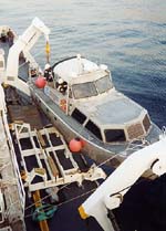
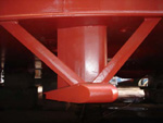
Multibeam Bathymetry

The NOAA Ship Thomas Jefferson, and two 8.5-m aluminum Jensen launches (3101 and 3102) deployed from the ship, acquired multibeam bathymetric data from the study area over an approximately 102-km² area during 2008 (figs. 6, 7, 8). The multibeam echosounder data were collected with hull-mounted RESON SeaBat 240-kilohertz (kHz) 8101 and 455-kHz 8125 shallow-water systems aboard the launches (figs. 9, 10) and a RESON duel frequency (200-kHz/400-kHz) 7125 system aboard the NOAA Ship Thomas Jefferson (fig. 11). Original vertical resolution of the multibeam bathymetric data was 0.5 m for water depths less than 20 m and 2 m for the deeper parts of the survey area. The bathymetric datasets were acquired in extended Triton data format (XTF), recorded digitally through an ISIS data acquisition system, and processed by NOAA using CARIS Hydrographic Image Processing System (HIPS) software for quality control, to incorporate sound velocity and tidal corrections, and combined into a 2-m grid to produce the final digital terrain model. A more detailed description of the acquisition parameters and processing steps performed by NOAA and the USGS to create the datasets presented in this report are included in the metadata files. These files can be accessed through the Data Catalog section of this report. Vertically exaggerated (5x), hill-shaded (illuminated from 0° north at an angle of 45°) imagery was created using CARIS HIPS software.

Horizontal positioning was by differential global positioning (DGPS) systems; Hypack MAX was used for acquisition line navigation. Sound-velocity corrections were derived with frequent conductivity-temperature-depth (CTD) profiles using a Sea-Bird Electronics, Inc., SEACAT CTD; casts were made with a Brooke Ocean Technology Moving Vessel Profiler 100 (fig. 12) from the Thomas Jefferson and with a small manually deployed CTD from the launches (fig. 13). Tidal zone corrections were calculated from data acquired by the National Water Level Observation Network stations at Newport, R.I., and Menemsha, Mass. The vertical datum is mean lower low water. Detailed descriptions of the MBES and sidescan-sonar acquisition and processing can be found in the descriptive report (National Oceanic and Atmospheric Administration, 2008).

Sampling and Photography

Most of the sediment sampling and bottom photography were conducted during July 2010 aboard the research vessel (RV) Rafael (fig. 14) during cruise 2010-033-FA; four additional stations were occupied during September 2010 aboard the RV Connecticut (fig. 15) during cruise 2010-005-FA. Surficial sediment samples (0-2 centimeters (cm) below the sediment-water interface) and (or) bottom photography were collected at 25 stations with a modified Van Veen grab sampler equipped with still- and video-camera systems (figs. 16, 17). The photographic data were used to appraise intra-station bottom variability, faunal communities, and sedimentary structures (indicative of geological and biological processes) and to observe boulder fields where samples could not be collected. Stations where textural interpretations were produced from the bottom photography include: 922-1, 922-3, 922-6, 922-7, 922-13, 922-14, 922-17, 922-18, and 922-20. A gallery of images collected as part of this project is provided in the Bottom Photography section; locations of the bottom photographs can be accessed through the Data Catalog section.

In the laboratory, the sediment samples were disaggregated and wet sieved to separate the coarse and fine fractions. The fine fraction (less than 62 microns) was analyzed by Coulter Counter, the coarse fraction was analyzed by sieving, and the data were corrected for salt content. Sediment descriptions are based on the nomenclature proposed by Wentworth (1922; fig. 18) and the size classifications proposed by Shepard (1954; fig. 19). A detailed discussion of the laboratory methods employed is given in Poppe and others (2005). Because biogenic carbonate shells commonly form in situ, they usually are not considered to be sedimentologically representative of the depositional environment. Therefore, gravel-sized bivalve shells and other biogenic carbonate debris were ignored. The grain-size analysis data can be accessed through the Data Catalog section of this report; a data dictionary is available in the Sediments section.

To facilitate interpretations of the distributions of surficial sediment and sedimentary environments, these data were supplemented by sediment data from compilations of earlier studies (Garrison and McMaster, 1966; Poppe and others, 2003; Poppe and others, 2005) and unpublished datasets from the National Geophysical Data Center. The interpretations of sea-floor features, surficial sediment distributions, and sedimentary environments presented herein are based on data from the sediment sampling and bottom photography stations, on tonal changes in backscatter on the imagery, and on the bathymetry. For the purposes of this paper, bedforms are defined by morphology and amplitude. Sand waves are higher than 1 m; megaripples are 0.2 to 1 m high; ripples are less than 0.2 m high (Ashley, 1990). The bathymetric grids and imagery released in this report should not be used for navigation.

To view files in PDF format, download a free copy of Adobe Reader.