 |
Figure 1. Index map showing the locations of the National Oceanic and Atmospheric Administration (NOAA) H12013 study area (red polygon) and the other bathymetric and backscatter surveys completed in Long Island Sound by NOAA and by the U.S. Geological Survey (USGS) and the Connecticut Department of Energy and Environmental Protection (CT DEEP). Surveys by the NOAA ships Thomas Jefferson and Rude are shown in light gray and include H11043 (Poppe and others, 2004, 2006a); H11044 (McMullen and others, 2005; Poppe and others, 2008a); H11045 (Beaulieu and others, 2005); H11255 (Poppe and others, 2006c); H11250 (Poppe and others, 2006b, 2007b); H11252 and H11361 (Poppe and others, 2007a, 2008b); H11441, H11442, H11224, and H11225 (Poppe and others, 2010a); H11445 (McMullen and others, 2010); H11251 (Poppe and others, 2010b); H11446 (McMullen and others, 2011); H11997 (Poppe and others, 2011a); H11999 (McMullen and others, 2012); and the combined contiguous datasets in eastern Long Island Sound (Poppe and others, 2011b). Sites of USGS sidescan-sonar surveys are shown in dark gray and include Norwalk (Twichell and others, 1997), Milford (Twichell and others, 1998), New Haven Harbor and New Haven Dumping Ground (Poppe and others, 2001), Roanoke Point (Poppe and others, 1999b), Falkner Island (Poppe and others, 1999a), Hammonasset (Poppe and others, 1997), Niantic Bay (Poppe and others, 1998c), New London (Lewis and others, 1998, Zajac and others, 2000, 2003), and Fishers Island Sound (Poppe and others, 1998b). |
 |
Figure 2. Map showing the major physiographic features in the vicinity of the study area, the extent of the multibeam bathymetric dataset (National Oceanic and Atmospheric Administration survey H12013), and the maximum strengths and directions of the flood and ebb tidal flows (White and White, 2012). |
 |
Figure 3. True-color image taken by the National Aeronautics and Space Administration (NASA) Thematic Mapper on the Landsat 5 satellite. Image shows plume of suspended sediment discharged by the Connecticut River into Long Island Sound after Hurricane Irene impacted New England during August 2011. Open polygon shows approximate location of study area. |
 |
Figure 4. Port-side view of the National Oceanic and Atmospheric Administration ship Thomas Jefferson at sea. The 8.5-m survey launch normally stowed on this side of the ship has been deployed. |
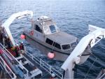 |
Figure 5. The National Oceanic and Atmospheric Administration (NOAA) launch 3102 being deployed from the NOAA ship Thomas Jefferson. |
 |
Figure 6. Starboard-side view of the National Oceanic and Atmospheric Administration launch 3102 at sea. |
 |
Figure 7. The RESON SeaBat 8125 multibeam echosounder hull-mounted to the National Oceanic and Atmospheric Administration launch 3101. |
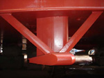 |
Figure 8. The RESON 7125 multibeam echosounder hull-mounted to the National Oceanic and Atmospheric Administration ship Thomas Jefferson. |
 |
Figure 9. Brooke Ocean Technology moving vessel profiler with a Sea-Bird Electronics, Inc. conductivity-temperature-depth (CTD) profiler used to correct sound velocities for the multibeam data collected aboard the National Oceanic and Atmospheric Administration ship Thomas Jefferson. |
 |
Figure 10. Sea-Bird Electronics, Inc. SEACAT conductivity-temperature-depth (CTD) profiler. Data derived from frequent deployments of this device were used to correct sound velocities for the multibeam data. |
 |
Figure 11. Comparison of the original reconnaissance multibeam bathymetry (above) and the interpolated and regridded bathymetry (below) for National Oceanic and Atmospheric Administration survey H12013. Panels on the left show the entire study area, open black polygons show locations of clips; panels on the right show clips of the enlarged bathymetry. |
 |
Figure 12. Detailed planar view comparing the original reconnaissance multibeam bathymetry (above) and the interpolated and regridded bathymetry (below) from National Oceanic and Atmospheric Administration survey H12013. Locations of views are shown in figure 21. |
 |
Figure 13. A Klein 5000 sidescan-sonar system hull-mounted to a National Oceanic and Atmospheric Administration launch. |
 |
Figure 14. A port-side view of the U.S. Geological Survey Research Vessel Rafael, which was used to collect bottom photography and sediment samples for this study. |
 |
Figure 15. Locations of stations at which bottom samples and photographs were taken during U.S. Geological Survey cruises 2009-059-FA and 2010-010-FA of Research Vessel Rafael to verify bathymetric and backscatter data. |
 |
Figure 16. The small Seabed Observation and Sampling System (mini-SEABOSS), a modified van Veen grab sampler equipped with still and video photographic systems, mounted on the aft starboard side of the U.S. Geological Survey Research Vessel Rafael. Note the winch mounted on the davit (left) and the take-up reel for the video-signal and power cable (right). |
 |
Figure 17. Correlation chart showing the relationships among phi sizes, millimeter diameters, size classifications (Wentworth, 1922), and American Society for Testing and Materials and Tyler sieve sizes. Chart also shows the corresponding intermediate diameters, grains per milligram, and settling and threshold velocities. |
 |
Figure 18. Sediment-classification scheme from Shepard (1954), as modified by Schlee (1973) and Poppe and others (2004b). |
 |
Figure 19. Digital terrain model of the sea floor produced from the multibeam bathymetry collected during National Oceanic and Atmospheric Administration survey H12013, gridded to 2 m and merged with the interpolated bathymetry data to give a more continuous perspective. Image is sun-illuminated from the northeast and vertically exaggerated fivefold. Warmer colors are shallower areas; cooler colors are deeper areas. |
 |
Figure 20. Interpretation of the digital terrain model from National Oceanic and Atmospheric Administration survey H12013. Areas of the sea floor characterized by rocks, sand waves, and megaripples are shown; white areas within the survey boundary are places where the sea floor is relatively smooth. |
 |
Figure 21. Locations of detailed planar views of the digital terrain model (yellow polygons) and profiles of bedform symmetry (green lines). Directions of net sediment transport (blue arrows), interpreted from obstacle marks and bedform asymmetry, are also shown. Profiles A-E are shown in figures 26 and 29. |
 |
Figure 22. Detailed planar view of the multibeam bathymetric data from National Oceanic and Atmospheric Administration survey H12013 off Hatchett Point. Image shows bedrock outcrops, scattered boulders, an obstacle mark indicating net westward sediment transport, and locations of stations OL3 and OL10. Location of view is shown in figure 21. |
 |
Figure 23. Detailed planar view of the multibeam bathymetric data from National Oceanic and Atmospheric Administration survey H12013 showing bedrock outcrops south of Hatchett Reef. Scour features around the outcrops indicate net westward sediment transport. Location of view is shown in figure 21. |
 |
Figure 24. Detailed planar view of the multibeam bathymetric data from National Oceanic and Atmospheric Administration survey H12013 showing Hatchett Reef. Image shows boulders scattered on and around the reef, bedrock outcrops, location of station OL9, and asymmetrical transverse and barchanoid bedforms indicating net southwestward sediment transport. White box is area where no data are available. Location of view is shown in figure 21. |
 |
Figure 25. Detailed planar view of the multibeam bathymetric data from National Oceanic and Atmospheric Administration survey H12013 showing part of the sand-wave field along the southern flank of Long Sand Shoal. Image shows that asymmetrical bedforms with transverse morphologies are dominant on the flanks, but that symmetrical bedforms are prevalent on the crest of the shoal. Location of view is shown in figure 21. |
 |
Figure 26. Cross-sectional views of sand waves produced from bathymetric data collected during National Oceanic and Atmospheric Administration survey H12013. Profile A is from the sand-wave field along the southwestern edge of the study area; profile B is from along the southern flank of Long Sand Shoal. Sand-wave asymmetry indicates southwestward net sediment transport; the presence of megaripples on stoss slopes suggests transport is active. Locations of profiles are shown in figure 21. |
 |
Figure 27. Detailed planar view of the multibeam bathymetric data from National Oceanic and Atmospheric Administration survey H12013 showing part of the sand-wave field along the southwestern edge of the study area. Image shows that both transverse and barchanoid morphologies are present and that megaripples occur along the northern edge of the field. Location of view is shown in figure 21. |
 |
Figure 28. Detailed planar view of the multibeam bathymetric data from National Oceanic and Atmospheric Administration survey H12013 showing the field of megaripples north of Long Sand Shoal and location of station OL17. Note the loss of resolution in the interpolated bathymetry. Location of view is shown in figure 21. |
 |
Figure 29. Cross-sectional views of sand waves produced from bathymetric data collected during National Oceanic and Atmospheric Administration survey H12013. Profile C shows that up-flank transport at the eastern end of Long Sand Shoal helps maintain the shoal; profile D shows that bedforms in the field of megaripples north of Long Sand Shoal are commonly symmetrical; and profile E shows that bedform asymmetry on the northern edge of the broad shoal west of Hatchett Reef indicates net southwestward transport. Locations of profiles are shown in figure 21. |
 |
Figure 30. Detailed planar view of the multibeam bathymetric data from National Oceanic and Atmospheric Administration survey H12013 showing the relatively flat character of the sea floor in the lower energy, more protected area northeast of Hatchett Point. White boxes are areas where no data are available. Location of view is shown in figure 21. |
 |
Figure 31. Sidescan-sonar imagery produced from data collected during National Oceanic and Atmospheric Administration survey H12013. Light tones indicate hard returns and generally coarser grained sediments; dark tones indicate softer returns and generally finer grained sediments. |
 |
Figure 32. Detailed view of the sidescan-sonar mosaic produced during National Oceanic and Atmospheric Administration survey H12013 showing high-backscatter targets interpreted to be rocky outcrops. The higher backscatter floor of a scour depression indicates coarser grained sediment. Location of view is shown in figure 21. |
 |
Figure 33. Detailed planar view of the sidescan-sonar mosaic produced during National Oceanic and Atmospheric Administration survey H12013 showing relatively straight to sinuous alternating bands of high and low backscatter (tiger-stripe pattern) indicative of transverse megaripples. Location of view is shown in figure 21. |
 |
Figure 34. Detailed planar view of the sidescan-sonar mosaic produced during National Oceanic and Atmospheric Administration survey H12013 showing high-backscatter bedforms on the north-central part of the study area. Bedforms may be composed of shell debris. Location of view is shown in figure 21. |
 |
Figure 35. Station locations from U.S. Geological Survey cruises 2009-059-FA and 2010-010-FA (circles) and historical data (squares; Poppe and others, 1998a) used to verify the acoustic data from National Oceanic and Atmospheric Administration survey H12013, color-coded for sediment texture. |
 |
Figure 36. Distribution of sedimentary environments based on the digital terrain model from National Oceanic and Atmospheric Administration survey H12013 and verification data from U.S. Geological Survey cruises 2009-059-FA and 2010-015-FA. Areas characterized by erosion or nondeposition, coarse bedload transport, and sorting and reworking are shown. |
 |
Figure 37. Hydroids, sponges, and red seaweed covering boulders at stations OL7 and OL9. Sessile fauna and flora commonly cover rocky areas of the sea floor in high-energy environments. Numbers shown next to station numbers are the image number as listed in the GIS Data Catalog section of this report. Station locations are shown in figure 15. |
 |
Figure 38. Gravel and gravelly sediment armors the sea floor in the high-energy environments between boulders at station OL9, around rocky areas at station OL3, and throughout much of the southern part of the study area. Numbers shown next to station numbers are the image number as listed in the GIS Data Catalog section of this report. Station locations are shown in figure 15. |
 |
Figure 39. Bottom photographs from stations OL13 and OL16 of current-rippled sand that is prevalent in areas with sedimentary environments characterized by processes associated with coarse-bedload transport. Numbers shown next to station numbers are the image number as listed in the GIS Data Catalog section of this report. Station locations are shown in figure 15. |
 |
Figure 40. Bottom photographs from stations OL1 and OL2 of the relatively flat- to faintly-rippled sea floor that is prevalent in areas with lower energy sedimentary environments characterized by processes associated with sorting and reworking. Numbers shown next to station numbers are the image number as listed in the GIS Data Catalog section of this report. Station locations are shown in figure 15. |
 |
Figure 41. Bottom photographs from stations OL11 and OL15 showing that shell beds armor much of the sea floor in the east-west trending depression that lies across the northern part of the study area. Numbers shown next to station numbers are the image number as listed in the GIS Data Catalog section of this report. Station locations are shown in figure 15. |
| |
Title Page Graphic. The graphic on the title page is a collage showing examples of a bottom photograph, clips of the hill-shaded bathymetry, and a bathymetric profile across sand waves. |


