 |
Figure 1. Index map showing the locations of the National Oceanic and Atmospheric Administration (NOAA) H12012 study area (red polygon) and the other bathymetric and backscatter surveys completed in Long Island Sound by NOAA and by the U.S. Geological Survey (USGS) and the Connecticut Department of Energy and Environmental Protection (CT DEEP). Surveys by the NOAA ships Thomas Jefferson and Rude are shown in light gray and include H11043 (Poppe and others, 2004a, 2006a); H11044 (McMullen and others, 2005; Poppe and others, 2008a); H11045 (Beaulieu and others, 2005); H11255 (Poppe and others, 2006b); H11250 (Poppe and others, 2006c, 2007b); H11252 and H11361 (Poppe and others, 2007a, 2008b); H11441, H11442, H11224, and H11225 (Poppe and others, 2010a); H11445 (McMullen and others, 2010); H11251 (Poppe and others, 2010b); H11446 (McMullen and others, 2011); H11997 (Poppe and others, 2011a); H11999 (McMullen and others, 2012); H12013 (Poppe and others, 2013); and the combined contiguous datasets in eastern Long Island Sound (Poppe and others, 2011b). Sites of USGS sidescan-sonar surveys are shown in dark gray and include Norwalk (Twichell and others, 1997), Milford (Twichell and others, 1998), New Haven Harbor and New Haven Dumping Ground (Poppe and others, 2001), Roanoke Point (Poppe and others, 1999b), Falkner Island (Poppe and others, 1999a), Hammonasset (Poppe and others, 1997), Niantic Bay (Poppe and others, 1998c), New London (Lewis and others, 1998, Zajac and others, 2000, 2003), and Fishers Island Sound (Poppe and others, 1998b). |
 |
Figure 2. Map showing the location of end moraines, submerged moraine lines in southern New York and New England (modified from Gustavson and Boothroyd, 1987), the extent of marine deltaic deposits from the Connecticut River (Lewis and DiGiacomo-Cohen, 2000), and the location of the study area (red polygon). The Ronkonkoma-Block Island-Nantucket end moraine represents the maximum advance of the Laurentide Ice Sheet about 20,000-24,000 years ago; the Harbor Hill-Roanoke Point-Charleston-Buzzards Bay end moraine represents a retreated ice-sheet position from about 18,000-21,000 years ago (Uchupi and others, 1996; Balco and others, 2002, Balco and others, 2009). |
 |
Figure 3. Port-side view of the National Oceanic and Atmospheric Administration ship Thomas Jefferson at sea. |
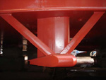 |
Figure 4. The RESON 7125 multibeam echosounder hull-mounted to the National Oceanic and Atmospheric Administration ship Thomas Jefferson. |
 |
Figure 5. Brooke Ocean Technology moving vessel profiler with a Sea-Bird Electronics, Inc. conductivity-temperature-depth (CTD) profiler used to correct sound velocities for the multibeam data collected aboard the National Oceanic and Atmospheric Administration ship Thomas Jefferson. |
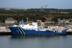 |
Figure 6. A port-side view of the U.S. Environmental Protection Agency Ocean Survey Vessel Bold that was used to collect bottom photography and sediment samples in the study area offshore in eastern Long Island Sound. |
 |
Figure 7. Locations of stations at which bottom samples and photographs were taken during U.S. Geological Survey cruises 2010-015-FA of Ocean Survey Vessel Bold and 2010-010-FA of Research Vessel Rafael to verify bathymetric and backscatter data. |
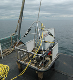 |
Figure 8. The mid-sized Seabed Observation and Sampling System (SEABOSS), a modified van Veen grab sampler equipped with still and video photographic systems designed and built by the U.S. Geological Survey. |
 |
Figure 9. Correlation chart showing the relationships among phi sizes, millimeter diameters, size classifications (Wentworth, 1922), and American Society for Testing and Materials (ASTM) and Tyler sieve sizes. Chart also shows the corresponding intermediate diameters, grains per milligram, and settling and threshold velocities. |
 |
Figure 10. Sediment-classification scheme from Shepard (1954), as modified by Schlee (1973) and Poppe and others (2004b). |
 |
Figure 11. Digital terrain model of the sea floor produced from the multibeam bathymetry collected during National Oceanic and Atmospheric Administration survey H12012, gridded to 2 m. Image is sun-illuminated from the northeast and vertically exaggerated fivefold. Warmer colors are shallower areas; cooler colors are deeper areas. |
 |
Figure 12. Interpretation of the digital terrain model from National Oceanic and Atmospheric Administration survey H12012. Areas of the sea floor characterized by rocky seabed, sand waves, megaripples, gravelly pavement, and dredge spoils are shown. |
 |
Figure 13. Locations of detailed planar views of the digital terrain model (yellow polygons) and profiles of bedform symmetry (green lines). Directions of net sediment transport (blue arrows), interpreted from obstacle marks and bedform asymmetry, are also shown. Profiles A to C are shown in figure 18. |
 |
Figure 14. Detailed planar view from the eastern part of the digital terrain model produced from bathymetric data collected during National Oceanic and Atmospheric Administration survey H12012 showing extensively exposed bedrock and location of station 012-25. Glacially smoothed bedrock ridges parallel similar features and glacial striations onshore (Goldsmith, 1962); strike ridges parallel those of the onshore Avalon terrane. Location of view is shown in figure 13. |
 |
Figure 15. Detailed planar view of the multibeam bathymetric data from National Oceanic and Atmospheric Administration survey H12012 showing relatively small bedrock outcrops on the basin floor south of Hatchett Point. Scour features around the outcrops indicate net westward sediment transport. Location of view is shown in figure 13. |
 |
Figure 16. Detailed planar view of the multibeam bathymetric data from National Oceanic and Atmospheric Administration survey H12012 showing broad scoured areas on the basin floor west of the extensive bedrock outcrops shown in figure 14 and the location of station 012-24. Mounded sediment along the western edge of these scoured areas indicates net westward sediment transport. Location of view is shown in figure 13. |
 |
Figure 17. Detailed planar view from the digital terrain model produced from bathymetric data collected during National Oceanic and Atmospheric Administration survey H12012 showing transverse sand waves on top of a shallow shelf platform and locations of stations 012-6 and 012-8. Note that the transition from the bordering relatively flat sea floor is abrupt and that megaripples progressively give way to sand waves. Location of view is shown in figure 13. |
 |
Figure 18. Cross-sectional views of transverse (profiles A and B) and barchanoid (profile C) sand waves from the digital terrain model produced from bathymetric data collected during National Oceanic and Atmospheric Administration survey H12012. Sand-wave asymmetry indicates westward net sediment transport; the presence of megaripples on stoss slopes suggests transport is active. Locations of profiles are shown in figure 13; vertical exaggerations of profiles A, B, and C are 54, 9, and 22, respectively. |
 |
Figure 19. Detailed planar view of relatively straight-crested, non-bifurcating transverse sand waves from the digital terrain model produced from bathymetric data collected during National Oceanic and Atmospheric Administration survey H12012. Note the presence of scour depressions or moats at the ends of the sand waves. Location of view is shown in figure 13. |
 |
Figure 20. Detailed planar view of barchanoid sand waves from the southwestern part of the digital terrain model produced from bathymetric data collected during National Oceanic and Atmospheric Administration survey H12012. Orientation indicates westward net sediment transport; also shown are an obstacle mark, the location of station 012-15, and the location of figure 21. Location of view is shown in figure 13. |
 |
Figure 21. Barchanoid sand waves originally surveyed in September–October 2008 during National Oceanic and Atmospheric Administration (NOAA) survey H11997 (open red polygons) and resurveyed in April–May 2009 during NOAA survey H12012 (open blue polygons). Note that the sand waves have shifted toward the west southwest. Location of figure is shown in figure 20. |
 |
Figure 22. Detailed planar view of dredge spoils of the Cornfield Shoals Disposal Site in the southwestern part of the digital terrain model produced from bathymetric data collected during National Oceanic and Atmospheric Administration survey H12012. Location of view is shown in figure 13. |
 |
Figure 23. Station locations from U.S. Geological Survey cruises 2010-010-FA and 2010-015-FA (circles) and historical data (squares; Poppe and others, 1998a) used to verify the acoustic data from National Oceanic and Atmospheric Administration (NOAA) survey H12012, color-coded for sediment texture. |
 |
Figure 24. Distribution of sedimentary environments based on the digital terrain model from National Oceanic and Atmospheric Administration (NOAA) survey H12012 and verification data from U.S. Geological Survey cruises 2010-010-FA and 2010-015-FA. Areas characterized by erosion or nondeposition, and coarse bedload transport are shown. |
 |
Figure 25. Hydroids, sponges, and hydrozoans covering boulders at stations 012-17c and 012-20c. Sessile fauna and flora commonly cover rocky areas of the sea floor in high-energy environments. Station locations are shown in figure 7. |
 |
Figure 26. Gravel and gravelly sediment armor the sea floor in the higher energy environments at stations 012-18b and 012-23c. These sediments are present around rocky areas and across much of the southern part of the study area. Station locations are shown in figure 7. |
 |
Figure 27. Bottom photographs from stations 012-5a and 012-3c showing shell beds typical of those that locally armor some of the sea floor. The beds are thin and composed primarily of mussels and mussel shell debris. Station locations are shown in figure 7. |
 |
Figure 28. Bottom photographs from stations 012-10a and 012-11a showing current-rippled sand that is prevalent in areas with sedimentary environments characterized by processes associated with coarse-bedload transport. Note the presence of scour depressions around gravel and shells. Station locations are shown in figure 7. |
 |
Figure 29. Bottom photograph from station 012-11b showing an outcrop of dense, pale red to gray mud interpreted to be part of the deltaic deposits that comprise the shallow shelf platform. Station location is shown in figure 7. |
 |
Figure 30. Locations of stations at which bottom photography was collected during U.S. Geological Survey cruises 2010-015-FA and 2010-010-FA to verify bathymetric data. |


