
In cooperation with the Michigan Department of Environmental Quality, Detroit Water and Sewerage Department, and the American Water Works Association Research Foundation
Scientific Investigations Report 2004–5072
Exemplary Results of Source Area Determinations
Model Development Needs and Limitations
Figure 1. The St. Clair-Detroit River Waterway in the Great Lakes Region.
Figure 2. Variogram of northing velocity components in the Marysville reach...
Figure 3. Relation between expected and simulated flows on St. Clair and D...
Figure 4. Relation between measured and simulated water levels on St. Clair...
Figure 5. Relation between expected and simulated easting velocity componen...
Figure 6. Relation between expected and simulated northing velocity compone...
Figure 7. Relation between expected and simulated easting velocity componen...
Figure 8. Relation between expected and simulated northing velocity compone...
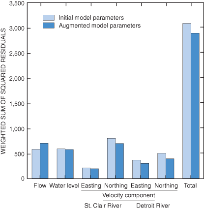
Figure 9. Uncertainty of flow, water level, and velocity simulations for th...
Figure 10. Variation of estimated Manning's n-values among material types f...
Figure 11. Variation of Manning's "n" value with depth for average non-vege...
Figure 12. Standard and public water intake model grid topologies near Bell...
Figure 13. Advective velocities simulated at model nodes near Belle Isle, M...
Figure 14. Monthly mean flows on St. Clair River and water levels at Bar Po...
Figure 15. Monthly flow duration characteristics of St. Clair River.
Figure 16. Relation between monthly mean flows of St. Clair River and water...
Figure 17. Winds characteristics on Lake St. Clair by sector.
Figure 18. Areas of wind and flow dominated effects on the St. Clair-Detroi...
Figure 19. Particle tracking results on St. Clair River near Port Huron, Mi...
Figure 20. Source areas for a selected point in L'anse Creuse Bay of Lake S...
Figure 21. Source areas for a selected point in L'anse Creuse Bay of Lake S...
Figure 22. Source areas for a selected point in L'anse Creuse Bay of Lake S...
Figure 23. Source areas for a selected point in L'anse Creuse Bay of Lake S...
Table 1. Primary boundary conditions used in model recalibration scenarios.
Table 2. Estimated parameter values for the hydrodynamic model of...
Table 3. Selected flow magnitudes on St. Clair River and water levels...
Table 4. Wind characteristics at the weather station on Lake St. Clair...
| Multiply | By | To obtain |
|---|---|---|
| Length | ||
| mile (mi) | 1.609 | kilometer (km) |
| International foot (ft) | 0.3048 (exactly) | meters |
| Area | ||
| acre | 0.4047 | hectare (ha) |
| square mile (mi2) | 2.590 | square kilometer (km2) |
| Volume | ||
| gallon (gal) | 3.785 | liter (L) |
| Flow rate | ||
| cubic foot per second (ft3/s) | 0.02832 | cubic meter per second (m3/s) |
Temperature in degrees Celsius (°C) may be converted to degrees Fahrenheit (°F) as follows:
°F=(1.8x°C)+32
DATUM
Vertical datum: The vertical datum currently used throughout the Great Lakes is the International Great Lakes Datum of 1985 (IGLD 85), although references to the earlier datum of 1955 are still common. This datum is a dynamic height system for measuring elevation, which varies with the local gravitational force, rather than an orthometric system, which provides an absolute distance above a fixed point. The primary reason for adopting a dynamic height system within the Great Lakes is to provide an accurate measurement of potential hydraulic head. The reference zero for IGLD 85 is a tide gage at Rimouski, Quebec, which is located near the outlet of the Great Lakes-St. Lawrence River system. The mean water level at the Rimouski, Quebec gage approximates mean sea level.
Horizontal datum: Horizontal distances in this report are referenced to the North American Datum of 1983 (NAD 83). The datum specifies a particular model for the shape of the earth, points of origin, and physical measurements to relate the specified point of origin to other points of origins. The datum provides a mechanism to translate a specific physical location to coordinates of latitude and longitude. Angular coordinates of latitude and longitude were projected from a spherical to a flat two-dimensional representation by use of the Michigan State Plane Coordinate System of 1983 (MSPCS 83), southern zone (2113). Although all such projections introduce some distortions, the MSPCS 83 introduces a distortion of less than one part in 10,000, and facilitates the measurements of lengths and distances based only on an Easting (x-coordinate) and Northing (y-coordinate).
Source areas to public water intakes on the St. Clair-Detroit River Waterway were identified by use of hydrodynamic simulation and particle-tracking analyses to help protect public supplies from contaminant spills and discharges. This report describes techniques used to identify these areas and illustrates typical results using selected points on St. Clair River and Lake St. Clair. Parameterization of an existing two-dimensional hydrodynamic model (RMA2) of the St. Clair-Detroit River Waterway was enhanced to improve estimation of local flow velocities. Improvements in simulation accuracy were achieved by computing channel roughness coefficients as a function of flow depth, and determining eddy viscosity coefficients on the basis of velocity data. The enhanced parameterization was combined with refinements in the model mesh near 13 public water intakes on the St. Clair-Detroit River Waterway to improve the resolution of flow velocities while maintaining consistency with flow and water-level data. Scenarios representing a range of likely flow and wind conditions were developed for hydrodynamic simulation. Particle-tracking analyses combined advective movements described by hydrodynamic scenarios with random components associated with sub-grid-scale movement and turbulent mixing to identify source areas to public water intakes.
The St. Clair-Detroit River Waterway connects Lake Huron with Lake Erie in the Great Lakes region and forms part of the international boundary between the United States and Canada. The waterway is a major navigational and recreational resource in the region, and provides a water supply for residents in both the United States and Canada. Thirteen public water intakes (PWIs) located on the U.S. side of the waterway provide water to about one quarter of the residents in Michigan.
The Michigan Department of Environmental Quality (MDEQ) initiated the Source Water Assessment Program (SWAP) to assess the susceptibility of public drinking water supplies to contamination. Together with the Detroit Water and Sewerage Department, and the American Water Works Association Research Foundation, MDEQ, and the U.S. Geological Survey has supported the development of a two-dimensional hydrodynamic model of the waterway and the application of particle-tracking analyses to identify source areas to the public water intakes. This report documents the techniques used in the analysis and illustrates the results for selected points.
This report was developed to document techniques used to identify source areas to PWIs within the St. Clair-Detroit River Waterway. Source areas are defined as areas within the waterway over which water passes on its way to the intakes. Because of extended retention times in some parts of the waterway, source areas were limited to those areas where the travel times from the origin to the intake would take less than 3 days. In addition, delimited source areas were generally limited to those areas, which were downstream of the next upstream PWI, or a model boundary, whichever was closer. Results were used to identify areas within the modeled waterway where PWIs are likely to be susceptible to contaminant spills and discharges.
The model developed in this report is based on a two-dimensional approximation to a flow system that may exhibit three-dimensional flow characteristics. In particular, velocity vectors in reaches with high flow velocities and significant channel curvature may not have the same direction over the entire water column at any instant of time as depicted when velocities are depth-averaged. Thus, any differences in source areas with depth of flow will not be accurately represented. Further, the model assumes a homogeneous fluid with a free surface. Simulations during periods of temperature stratification or ice cover would be of uncertain reliability.
St. Clair River, Lake St. Clair, and Detroit River form a waterway that is part of the international boundary between the United States and Canada (fig. 1). The waterway, which connects Lake Huron with Lake Erie, is a major navigational and recreational resource of the Great Lakes basin. St. Clair River (the upper connecting channel) extends about 39 mi from its headwaters at the outlet of Lake Huron near Port Huron, Michigan, to an extensive delta area. Throughout its length, water levels (water-surface elevations) decrease about 5 ft as it discharges an average of 182,000 ft3/s from a drainage area of about 222,400 mi2. Local tributaries to St. Clair River include Black River at Port Huron, Michigan, Pine River at St. Clair, Michigan, and Belle River at Marine City, Michigan. Lake St. Clair receives water from St. Clair River, and lesser amounts from Clinton River in Michigan and the Thames and Sydenham Rivers in Ontario, Canada. Along the 25-ft deep navigational channel, the lake has a length of 35 mi. The lake's round shape, with a surface area of 430 mi2, and shallow depths that average about 11 ft, make its exposure to winds similar in all directions. Detroit River (the lower connecting channel) receives water from Lake St. Clair and lesser amounts from River Rouge in Michigan, where it flows 32 mi to Lake Erie. Water levels fall about 3 ft within Detroit River, which has an average flow of about 186,000 ft3/s.
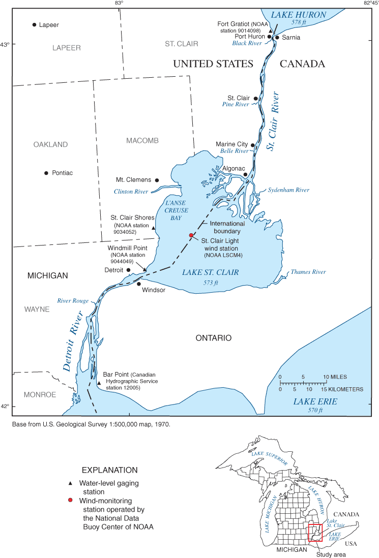
Figure 1. The St. Clair-Detroit River Waterway in the Great Lakes Region.
Numerous investigators have contributed to the understanding of flow on the St. Clair-Detroit River Waterway. Schwab and others (1989) compared currents measured on Lake St. Clair with particle-tracking results computed based on two-dimensional hydrodynamic simulations. Tsanis, Shen, and Venkatesh (1996) implemented RMA2 on St. Clair and Detroit Rivers; results indicated that simulated currents closely matched field measurements of drifting buoys. Williamson, Scott, and Lord (1997) developed a two-dimensional finite-element model of the St. Clair-Detroit River system for the Canadian Coast Guard for water-level prediction and assessment of structures in the river systems. The U.S. Army Corps of Engineers (USACE) Waterway Experiment Station (WES) in Vicksburg, Mississippi developed a prototype two-dimensional model of the St. Clair-Detroit River waterway for the Detroit District USACE (Ron Heath, USACE-WES, written commun., 1999). The resulting model was modified and adapted for use in a joint study by Environment Canada and the Detroit District USACE, to assess the effects of encroachments on water levels in St. Clair and Detroit Rivers (Aaron Thompson, Environment Canada, written commun., July 2000). A two-dimensional hydrodynamic model was initially applied to the St. Clair-Detroit River Waterway by matching water-surface elevations and flows in numerous branches to measured values (Holtschlag and Koschik, 2002).
Hydrodynamic simulations and particle-tracking analyses were used to identify source areas to selected PWIs on the St. Clair-Detroit River Waterway. A hydrodynamic model (RMA2) of the St. Clair-Detroit River (Holtschlag and Koschik, 2002) was developed to simulate flows and water levels in major branches of the waterway. This model was recalibrated to more accurately simulate the distribution of flow velocities within the branches based on acoustic Doppler current profiler (ADCP) surveys of St. Clair and Detroit Rivers. Once recalibrated, the finite element mesh was refined to improve the spatial resolution of flows near PWIs. Hydrodynamic simulations using the refined mesh were used to determine the advective components of flow for a wide range of flow, water-level, and wind conditions. By reversing the signs of the simulated velocity fields and adding a random component associated with turbulent mixing, particle-tracking analyses were used to identify source areas to public water intakes.
Hydrodynamic simulations were used to determine the advective components of flow, or those average velocity components that can be expected to occur for specified flow, water level, and wind boundary conditions, given the geometry and hydraulic characteristics of the waterway. Hydrodynamic simulations were developed using the generalized computational code RMA2-WES (referred to as RMA2 in this report) to solve the two-dimensional equations of flow (Donnell and others, 2003). The Surface water Modeling System (SMS), a computer program for surface water model development, was used to create input files describing the waterway in a form that is suitable for simulation with RMA2, and for post processing and displaying hydrodynamic simulation and particle tracking results. Selected aspects of the generalized hydrodynamic model are discussed in the following paragraphs.
RMA2 is a generalized FORTRAN (Formula Translation) computer code for two-dimensional hydrodynamic simulation of surface-water bodies. The code facilitates the computation of horizontal flow-velocity components and water levels (water-surface elevations) for subcritical, free-surface flow. RMA2 implements a finite-element solution of the Reynolds form of the Navier–Stokes equations for turbulent flows. Donnell and others (2003) provide detailed documentation of the governing equations, their solution by the finite element method, and recommended uses and limitations of the RMA2 code. RMA2 is under continual development by the U.S. Army Corps of Engineers at the Waterway Experiment Station, Coastal Hydraulics Laboratory in Vicksburg, Miss. In this report, RMA2 version 4.55, which was last modified on July 30, 2003, was used for the simulations.
A brief overview of those modeling aspects needed to help understand the source water identification process is provided subsequently. To solve the partial differential-flow equations numerically, the waterway area is discretized into a mesh of quadrilateral and triangular elements defined at points by nodes. The finite element discretization provides a flexible representation of an irregularly shaped waterway. Nodes are located at the vertices of elements and at midside edges connecting nodes. Thus, eight nodes are defined per quadrilateral element, and six nodes are defined per triangular element. Contiguous elements forming branches or subreaches of the waterway are grouped into material zones to facilitate characterization of the waterway. Channel-roughness coefficients and eddy viscosity characteristics are assigned to material zones.
Hydrodynamic simulations compute water levels and flow velocities at interior nodes on the basis of boundary conditions specified at exterior nodes, the hydraulic characteristics of the waterway, and the flow equations. Boundary conditions include flow (discharge across one or more elements), water level, and wind conditions. Quadratic interpolation is used to determine water levels and velocities anywhere within the elemental areas based on nodal values. Thus, greater densities of nodes provide improved spatial resolution of velocity fields, but also require additional computational resources.
Velocity distributions are largely determined by the advection component described by hydrodynamic simulation. Water velocities may decrease in shallow areas due to aquatic vegetation that effectively increases channel roughness, and adjacent points may have more or less similar velocities based on the effectiveness of turbulent exchange in mixing the water. Neither channel roughness nor turbulent exchange, which is the fluid momentum transfer due to chaotic motions of fluid particles (Donnell and others, 2003), can be measured directly in the field, but can be inferred from measurements of flow, water level, and velocity.
To reproduce observed variations in the velocity distributions with RMA2, local velocities V may be computed by use of the Manning's equation, where Manning's channel roughness coefficient (Manning's "n") is expressed in English units of measurement as a function of flow depth as:
In RMA2, Manning's "n" may be described as a monotonically decreasing function of flow depth (Donnell and others, 2003) as:
RDR0k, RDCOEF, RDRM, and RDD0 were unknown model parameters inferred by calibration. In RMA2, the eddy viscosity coefficient represents the effects of both molecular viscosity and turbulence on turbulence exchange, in which the turbulence component normally dominates. In general, turbulence exchanges depend on the momentum of the flow, spatial gradients of the velocity, and the scale of the flow phenomenon, as described by the length of the element in the direction of flow. For consistency with the physical system, eddy viscosity coefficients in the mesh should increase with element size and flow velocity. Higher eddy viscosities are associated with greater uniformity of velocity distributions across a channel segment.
Although eddy viscosities may be assigned directly to elements in material zones, greater consistency and flexibility is obtained within RMA2 by assigning eddy viscosities to elements on the basis of the Peclet formula (Donnell and others, 2003), in which the Peclet number is inversely related to the eddy viscosity as:
The Surface-Water Modeling System (SMS) is a computer program for pre- and post-processing selected surface-water models, including RMA2. Environmental Modeling Research Laboratory (2003) provides detailed documentation of the program. Holtschlag and Koschik (2002) document the use of SMS in developing an earlier version of the RMA2 model for the St. Clair-Detroit River Waterway.
Development of a RMA2 hydrodynamic model to identify source areas to public water intakes on the St. Clair-Detroit River Waterway began in 1999 as part of the MDEQ Source Water Assessment Program. The initial model version (Holtschlag and Koschik, 2002) was calibrated to match water levels and flows through the major branches in the waterway. In this report, the initial version is recalibrated to describe the distribution of velocities within the St. Clair and Detroit Rivers based on acoustic Doppler current profiler (ADCP) surveys of flow velocities, while maintaining consistency with previously used flow and water-level data. To facilitate a computationally intensive calibration process, the recalibrated model version maintained the mesh design of the initial version. The recalibrated model is now considered the standard version, and supersedes the initial version of the model. Additional resolution of flow patterns and details on flow geometry near public water intakes were needed to identify source-water areas. Therefore, the mesh was refined to complete the assessments. The refined mesh with the recalibrated parameters from the standard version is referred to as the public water intake version. The public water intake version does not supersede the standard version, but provides an alternative formulation for situations requiring the enhanced flow resolution near public water intakes.
The initial version of the St. Clair-Detroit River flow model (Holtschlag and Koschik, 2002), discretized the St. Clair-Detroit River Waterway into 13,783 quadratic elements defined by 42,936 nodes. Sets of continguous elements were grouped into 25 material zones describing possible variations in effective channel roughness among branches in the waterway.
Seven steady-state scenarios were used in model calibration. These calibration scenarios are idealized hydraulic conditions associated with selected flow measurement events that were developed to efficiently calibrate the model throughout a wide range of flow and water-level conditions. Scenarios use steady-state simulations to approximate transient flow and water-level conditions during 3-to-4 day flow-measurements events. This approach reduces computational requirements to feasible levels with available computer resources. The approach is applicable to the St. Clair-Detroit River Waterway because the system is not tidally affected, and it is bounded by Lake Huron and Lake Erie, which can remain at fairly-constant levels for several days. In addition, simulating transient flow conditions on the St. Clair-Detroit River Waterway is currently problematic because the flow boundary at the head of St. Clair River cannot be determined reliably for transient conditions. Specifically, stage-fall-discharge ratings (Koschik, USACE, written commun., 2001) are only applicable to steady-state conditions.
UCODE (Poeter and Hill, 1998), an inverse modeling code, was used to systematically adjust model parameters, and to determine their associated uncertainty and correlation by use of nonlinear regression. Calibration results showed close agreement between simulated and expected flows in major channels and water levels at gaging stations. Resulting effective channel-roughness coefficients were within their plausible physical ranges. Some of the variations in effective channel roughness coefficients may be attributable to the discretization of the waterway and the sampled bathymetry data, rather than to actual differences in channel roughness characteristics. Eddy viscosities in the initial model version were assigned on the basis of the Peclet formula. A Peclet number of 15 was assigned to all material zones, which is within the recommended range of 15-40 (Donnell and others, 2003).
Model calibration is a process of adjusting model parameters to improve the match between simulated and measured, or expected, values. In this report, calibration efforts were focused on improving the accuracy of simulated velocities, while maintaining consistency with expected flows (total discharges) in major branches, and the water levels near gaging stations used in the initial calibration.
As in the initial model development, the universal inverse modeling code, UCODE, was used to estimate model parameters. Specifically, the maximum Manning's "n" values for non-vegetated water (RDR0k) were estimated for the 25 material zones defined in the initial model version. In addition, three model parameters (RDCOEF, RDRM, and RDD0) were defined to approximate the nonlinear variation of Manning's "n" with flow depth (Equation 2).
In the recalibration effort, eddy viscosities were initially based on a parameterization of the Smagorinski method (Donnell and other, 2003). The Smagorinski method provides time-dependent adjustments of eddy viscosities based on simulated velocities. The strength of this method over the Peclet method is that it takes into account the gradients of velocity to determine the appropriate turbulence coefficient to meet conditions in the hydrodynamic simulation. Although parameter estimation converged while simultaneously estimating the Manning's "n" coefficients and the Smagorinski-related parameters, numerical instabilities arose in the transfer of these parameters to the refined grid developed for source-water assessment. Therefore, the Smagorinski method and associated parameters were replaced with the Peclet method. Fixing the Manning's "n" coefficients at those values determined under the Smagorinski parameterization, final parameter estimation was used to determine a single Peclet number for the entire waterway.
UCODE, a universal code for parameter estimation (Poeter and Hill, 1998), was used to (1) manipulate RMA2 input and output files, (2) execute RMA2 with different parameter sets, (3) compare simulated with expected values, (4) apply a nonlinear regression code (Hill, 1998) to adjust parameter values in response to the comparison, (5) generate statistics for use in evaluating the uncertainty and correlation structure of estimated parameters, and (6) identify the contribution of individual observations or observation sets on parameter estimates through the sensitivity coefficients.
Parameter estimation with UCODE proceeds through a set of iterations until the user-specified criteria for convergence is attained or the specified maximum number of iterations is completed. In this report, convergence criteria specified that either the maximum parameter change be less than 0.5 percent or that the differences in the sum of squared weighted residuals change by less than 0.5 percent over three iterations. The criterion for satisfactory depth convergence in RMA2 was 0.002 ft in 10 iterations.
Within a single UCODE iteration, each parameter is, in turn, changed (perturbed) by a maximum of 2.5 percent, while the remaining parameters are held constant at their initial values or the values estimated at the end of the previous iteration. RMA2 is executed for each unique parameter set to complete the iteration. When a UCODE iteration is completed, parameter sensitivities are calculated for each observation as the ratio of change in corresponding simulated values to the change in parameter values. These sensitivities together with the model residuals are used with nonlinear regression to update all parameter estimates simultaneously for the beginning of the next iteration. Iteration continues until parameter estimation converges or the maximum number of specified iterations is exceeded.
Recalibration data included all flow and water-level data used in the development of the initial model version (Holtschlag and Koschik, 2002), plus velocity data obtained from ADCP surveys of St. Clair and Detroit Rivers. Flow-calibration data were expressed as expected values, which were based on the average flow measured in non-branched channel segments during the corresponding measurement interval (scenario), and the expected distribution of flows in the St. Clair-Detroit River Waterway (Holtschlag and Koschik, 2001). Water-level calibration data were the average of values measured during the period represented by the calibration scenario. Velocity estimates were based on interpolations from ADCP surveys.
The first ADCP survey (Holtschlag and Koschik, 2003a) was conducted on St. Clair River in June of 2002, and provides 2.7 million velocity measurements at 104 cross sections. Sections are spaced about 1,630 ft apart along the river from Port Huron to Algonac, Michigan, a distance of 28.6 mi. Two transects were obtained at each cross section, one in each direction across the river. Along each transect, ensembles of velocity measurements (a velocity profile) were obtained 2-4 ft apart. At each ensemble, average easting-, northing-, and vertical-velocity components were obtained for bins of water about 1.64 ft in height, beginning about 3 ft below the water surface and ending about 3 ft above the channel bottom.
The second ADCP survey (Holtschlag and Koschik, 2003b) was conducted on Detroit River from July 8-19, 2002. In this survey, more than 3.5 million velocities were measured at 130 cross sections. Cross sections were generally spaced about 1,800 ft apart along the river from the head of Detroit River at the outlet of Lake St. Clair to the mouth of Detroit River on Lake Erie. Again, two transects were surveyed at each cross section, one in each direction across the river. Along each transect, velocity ensembles were generally obtained 0.8-2.2 ft apart. At each ensemble, average water velocity data were obtained at 1.64 ft intervals of depth. Velocity and ancillary data from the St. Clair River and Detroit River surveys can be obtained through the internet at Web sites http://mi.water.usgs.gov/pubs/OF/OF03-119/ and http://mi.water.usgs.gov/pubs/OF/OF03-219/, respectively.
During both the St. Clair and Detroit River ADCP surveys, aquatic vegetation was encountered. In some areas, thick mats of aquatic vegetation prevented access to near-shore or other shallow areas by boat. In these areas, the ADCP survey transects were terminated at the edges of the aquatic mats, as point velocity data was of primary interest. The velocity distributions within the waterway are thought to be impacted by the seasonal aquatic growth. A single survey on each connecting channel, however, could not be used to quantify a seasonal variation.
Data processing was required to use data from ADCP surveys for model calibration. First, for consistency with the two-dimensional flow assumptions, the ADCP velocity data for all depth intervals were averaged at each ensemble, producing a single depth-averaged estimate of easting- and northing-velocity components at each velocity profile. Vertical-velocity components were not considered. To facilitate statistical analyses, depth-averaged velocity data in five or more transects were generally compiled for subreaches in which the International boundary is a straight-line segment. On St. Clair River, 15 channel segments were defined, and on Detroit River, 25 channel segments were defined. Each channel segment typically contained more than 11,000 depth-averaged velocity measurements.
The statistical analysis technique of kriging (Cressie, 1991) was used to estimate the easting and northing velocity components at model nodes on the basis of the ADCP velocity data. Kriging is a best linear unbiased estimator that computes the magnitude and uncertainty of a spatially-referenced quantity as a weighted average of nearby measured values. Sample weights are determined on the basis of the spatial-correlation structure and the configuration of measured values near the point of estimation.
Variogram analysis (Cressie, 1991) is commonly used to quantify the spatial-correlation structure for kriging estimation. In variogram analysis, separation distances between all possible measurement pairs are computed and the results divided into bins or lags of generally equal intervals of separation distances. In this analysis for example, all pairs of measurements that were within 2 ft of one another were included in the 1-foot bin or lag; measurements that were separated by a distance of 8 to 10 ft were included in the 9-foot lag distance; measurements that were separated by more than 100 ft were ignored. Within each lag, squared differences between all measured velocities were computed, and the average squared-differenced value was plotted at the center of each bin (fig. 2). In this analysis, each 2-foot bin commonly contained 20,000 or more measurement pairs. The set of averages of the squared-differenced values is referred to as the empirical variogram.
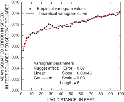
Figure 2. Variogram of northing velocity components in the Marysville reach of St. Clair River.
The empirical variogram quantifies the generally increasing similarity between velocity measurements at decreasing lag distances. Thus, velocity measurements that are 2 ft apart tend to be more similar in magnitude (have smaller average squared differences) than velocity measurements 100 ft apart. Because of temporal variations in velocities and measurement uncertainties, however, average squared-velocity differences do not necessarily tend to zero at zero separation distances.
For mathematical reasons, kriging estimation requires a slightly different description of the correlation structure than that provided directly by the empirical variogram. For this description, one or more theoretical variogram models are fit to the empirical variogram. In the variogram shown in figure 2, a nugget, a linear, and a Gaussian variogram model (Cressie, 1991) were combined to approximate the empirical variogram. In particular, the nugget component describes a discontinuity in the spatial correlation structure between zero and a slightly positive separation distance. The linear and Gaussian model components account for increases in the variogram (decreases in correlation) with increasing separation distance. The composite theoretical variogram was then used in the kriging equations (Cressie, 1991) to weight ADCP velocity measurements for estimation of velocities at model nodes. In this analysis, only velocity data that occurred within 100 ft of a model node was used in estimating velocity characteristics at the node.
Recalibration required integration of information on flows, water levels, and velocities. These calibration data are expressed in different units of measurements and include different numbers of observations. Specifically, 217 flow measurements, in cubic feet per second, and 121 water-level measurements, in feet, were used to match simulated flow and water-level values. In contrast, easting and northing velocity components, in feet per second, were estimated at 1,406 model nodes on St. Clair River, and 1,103 model nodes on Detroit River. This provides 5,018 velocity estimates (counting both northing and easting components) for comparison with simulated values.
To help reconcile disparate units of measurement, a weighting factor was determined that was inversely proportional to the variance (standard deviation squared) of the measurement, expressed in a consistent unit. Thus, larger standard deviations correspond to smaller weighting factors. To balance the relatively large number of velocity measurements with respect to smaller numbers of flow and water level measurements, the standard deviations of velocity values estimated by use of kriging were arbitrarily set equal to twice their estimated values.
Calibration scenarios are idealized hydraulic conditions associated with selected flow measurement events that were developed to efficiently calibrate the model throughout a wide range of flow and water-level conditions. Scenarios use steady-state simulations to approximate transient flow and water-level conditions during flow-measurements events. This approach reduces computational requirements to feasible levels with available computer resources.
All seven scenarios (table 1) used in the initial model calibration were used in model recalibration. The initial scenarios (1 through 7) were used exclusively to match flow and water-level information within the waterway, and applied exactly as previously described (Holtschlag and Koschik, 2002). Two scenarios were added to simulate conditions during the ADCP velocity surveys of St. Clair and Detroit Rivers. Scenarios 8 and 9 were used exclusively to match kriged velocity estimates and simulated velocities at model nodes.
Table 1. Primary boundary conditions used in model recalibration scenarios.
| Scenario | Dates of flow measurement event | Expected flow near the headwaters of St. Clair River at Fort Gratiot (in cubic feet per second) | Expected water level near the mouth of Detroit River at Bar Point, Ontario (in feet above IGLD 1985) |
|---|---|---|---|
| 1 | Nov. 3–5, 1999 | 173,201 | 570.052 |
| 2 | Oct. 26–29, 1998 | 194,065 | 571.591 |
| 3 | July 8–10, 1996 | 217,259 | 572.884 |
| 4 | Aug. 4–6, 1997 | 222,539 | 573.770 |
| 5 | Sep. 23–24, 1999 | 174,993 | 570.710 |
| 6 | May 5–7, 1997 | 213,719 | 573.498 |
| 7 | Sep. 21–24, 1998 | 197,907 | 572.271 |
| 8 | May to June, 2002 | 181,000 | 572.200 |
| 9 | July 8–19, 2002 | 173,800 | 572.100 |
Recalibration results indicate that a consistent relation (fig. 3) was maintained between simulated flows and flows expected based on an extensive set of field measurements and regression analyses (Holtschlag and Koschik, 2001). Over the range of flows in all branches, the average and standard deviation of percent errors between expected and simulated flows was –3.30 percent and 8.47 percent, respectively. Similarly, consistency was maintained between measured and simulated water levels (fig. 4), with a residual (difference between simulated and measured values) mean and standard deviation of 0.019 ft and 0.211 ft, respectively.
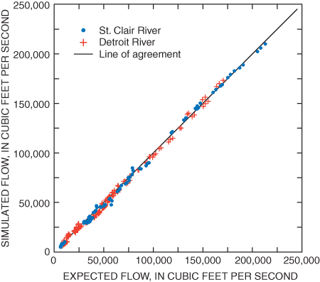
Figure 3. Relation between expected and simulated flows on St. Clair and Detroit River.
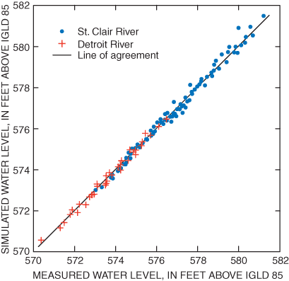
Figure 4. Relation between measured and simulated water levels on St. Clair and Detroit Rivers.
On St. Clair River, the mean and standard deviation of residuals between simulated and expected easting velocity components was –0.032 ft/s and 0.326 ft/s, respectively (fig. 5). Similarly, the mean and standard deviation of St. Clair River northing velocity residuals was –0.008 ft/s and 0.649 ft/s, respectively (fig. 6). On Detroit River, the mean and standard deviation of residuals of easting velocity components was –0.003 ft/s and 0.304 ft/s, respectively (fig. 7). Finally, the mean and standard deviation of residuals of northing velocity components on Detroit River was –0.004 ft/s and 0.379 ft/s, respectively (fig. 8). In comparison to the initial calibration results, recalibration with the augmented parameter set and additional velocity data indicates that accuracy of flow estimates may be degraded slightly, while the accuracy of water level and velocities may be enhanced under the new parameterization (fig. 9).
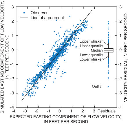
Figure 5. Relation between expected and simulated easting velocity components on St. Clair River.
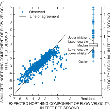
Figure 6. Relation between expected and simulated northing velocity components on St. Clair River.
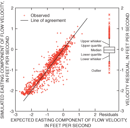
Figure 7. Relation between expected and simulated easting velocity components on the Detroit River.
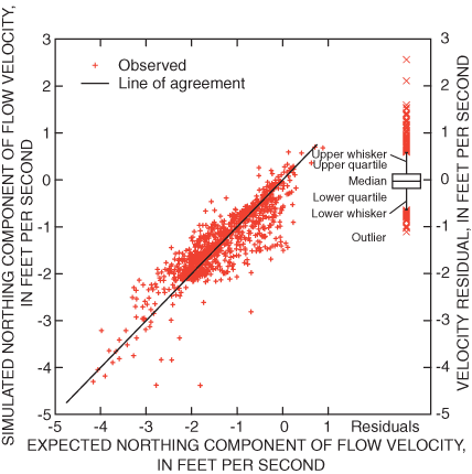
Figure 8. Relation between expected and simulated northing velocity components on the Detroit River.
The recalibrated hydrodynamic model of the St. Clair-Detroit River Waterway includes 29 parameters (table 2). Parameter estimation occurred in logarithmic space, rather than arithmetic space. Thus, when estimated parameters were transformed to arithmetic space (exponentiated) for hydrodynamic simulation, only positive values were possible. This constraint is consistent with the physically plausible range of the parameters.
| Parameter identifier (Subscripts for RDD0 identify material zones) | Augmented Parameter Set | Original Parameter Set: Expected value | Material zone group designation | |||
|---|---|---|---|---|---|---|
| Upper 95 percent confidence limit | Expected value | Lower 95 percent confidence limit | Composite scaled sensitivity | |||
| RDR01,2,38 | 0.039 | 0.0367 | 0.035 | 2.16 | 0.0290 | SCRUpper |
| RDR03,4,39 | .025 | .0230 | .021 | 1.92 | .0217 | SCRDryDoc |
| RDR05,6 | .030 | .0291 | .028 | 5.35 | .0255 | SCRDunnPap |
| RDR08,11 | .024 | .0231 | .022 | 3.54 | .0185 | SCRAlgonac |
| RDR014 | .051 | .0456 | .041 | 1.06 | .0419 | SCRFlats |
| RDR07 | .027 | .0255 | .024 | 1.98 | .0227 | SCRFawnIsE |
| RDR040 | .012 | .0103 | .009 | 1.50 | .0137 | ChenalEcar |
| RDR012 | .027 | .0254 | .024 | 2.41 | .0213 | SCRNorth |
| RDR013 | .023 | .0212 | .020 | 1.27 | .0203 | SCRMiddle |
| RDR015 | .041 | .0360 | .031 | .95 | .0316 | SCRCutoff |
| RDR016 | .027 | .0238 | .021 | .75 | .0270 | BassettCh |
| RDR017,18,19 | .018 | .0156 | .013 | 1.30 | .0265 | LakStClair |
| RDR020,41 | .031 | .0274 | .024 | 3.79 | .0314 | DETUpper |
| RDR022 | .030 | .0272 | .025 | 3.64 | .0305 | DETBelleIN |
| RDR025,42 | .030 | .0277 | .025 | 5.79 | .0084 | DETRRouge |
| RDR026-29 | .037 | .0330 | .029 | 4.93 | .0332 | DETFightIs |
| RDR043 | .027 | .0243 | .022 | 1.02 | .0345 | DETStonyIs |
| RDR035 | .041 | .0396 | .038 | 2.80 | .0373 | DETTrenton |
| RDR036,37 | .060 | .0560 | .052 | 1.92 | .0514 | DETSugarW |
| RDR046,48 | .073 | .0648 | .058 | .78 | .0660 | DETBobloIs |
| RDR032 | .041 | .0377 | .035 | 1.67 | .0314 | DETLivChLo |
| RDR044 | .010 | .0071 | .005 | .72 | .0148 | DETLivChUp |
| RDR033 | .016 | .0140 | .013 | 1.74 | .0217 | DETAmhChUp |
| RDR045 | .043 | .0411 | .039 | 3.26 | .0345 | DETAmhChLo |
| RDR047 | .045 | .0375 | .031 | .59 | .0226 | DETSugarE |
| RDD0 | 3.160 | 2.6286 | 2.190 | .50 | NA | NA |
| RDRM | .069 | .0546 | .043 | .84 | NA | NA |
| RDCOEF | .042 | .0320 | .025 | 3.08 | NA | NA |
| PECLET | 22.900 | 21.9010 | 21.000 | 1.46 | NA | NA |
Confidence limits are provided for estimated parameters, but may only indicate a relative uncertainty about their true values. Positive correlations among observations may reduce the effective number of measurements by an amount that is difficult to characterize. Lack of independence among measurements would widen confidence intervals from those that are computed assuming independence. Furthermore, confidence limits are based on the assumption of normally distributed residuals in logarithmic space. One indication of this normality, the correlation between weighted residuals and normal order statistics, is 0.798, which is lower than 0.987 that would be expected 95 percent of the time if the weighted residuals were normally distributed. Exponentiation of confidence limits computed for parameters in logarithmic space, results in some asymmetry in the confidence interval about the expected values in arithmetic space.
Of the 28 parameters associated with channel roughness (fig. 10), a high positive correlation of 0.98 exists between values for material zones DETUpper and DETBelleIN. This correlation indicates that some ambiguity may exist between these two parameters. In this case, however, the ambiguity is not thought to seriously degrade the estimates because the magnitudes of the two parameters are similar, and both values are within a physically plausible range. No other parameter pair had a correlation greater than 0.80, indicating that other ambiguities are unlikely. Material zones, which were initially numbered consecutively, were grouped during calibration. In this grouping, some material zones were assimilated into the material zones identified in table 2. Material zones may be viewed in SMS by downloading the geometry file (http://mi.water.usgs.gov/pubs/WRIR/WRIR01-4236/docs/SCDFlowModelInput.php).
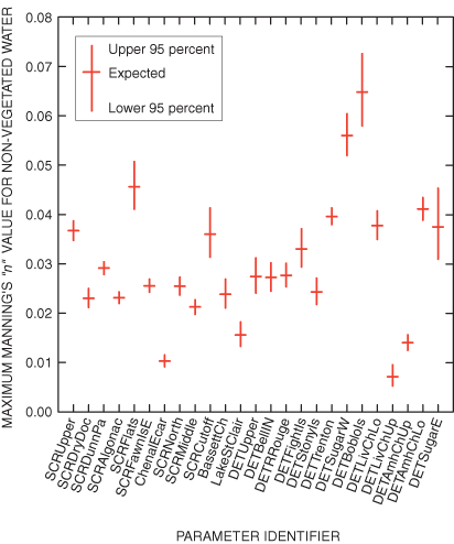
Figure 10. Variation of estimated Manning's n-values among material types for non-vegetated water.
Estimated values for RDD0, RDRM, and RDCOEF (Equation 1) in this report were near the ranges used in other studies noted by Donnell and others (2003) on the Mississippi River Delta and San Francisco Bay. In particular, the estimated value for RDD0 of 2.6286 was within the noted range of 2 to 4 ft. The RDRM value of 0.0546 was above the 0.026 to 0.040 range, and the RDCOEF value of 0.0320 was below the range of 0.080 to 0.167 (fig. 11). The estimated value for the Peclet number of 21.9 is within the expected range of 15 and 40.
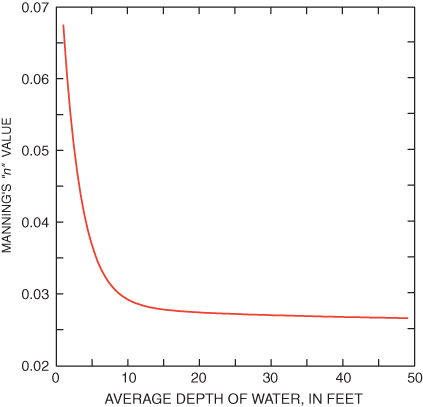
Figure 11. Variation of Manning's "n" value with depth for average non-vegetated surfaces.
A PWI version of the hydrodynamic model of the St. Clair Detroit River Waterway was developed specifically for source-water assessment. The PWI version inherits the parameterization of the recalibrated (standard) version, and includes mesh refinements that provide greater resolution of flows near public water intakes. Refinements generally were implemented by subdividing elements in the standard version into four equal sub-elements. Due to the density of PWIs in St. Clair River, nearly all the elements describing this river were refined. In other areas, refinements required the addition of elements not represented in the standard (initial) version. Figure 12 shows the addition and refinement of model elements near Belle Isle, Michigan on Detroit River where node additions provide a mechanism to simulate flows through a bypass channel south of the lagoon. Flows near the entrance to the lagoon also are simulated with greater resolution. Finally, element refinements were used to smooth the boundaries of the mesh, which facilitated the particle-tracking analyses.
The PWI version of the model contains 30,306 quadratic elements defined by 90,386 nodes, or more than twice as many elements and nodes as the standard version. Computer execution times and memory requirements are similarly increased.
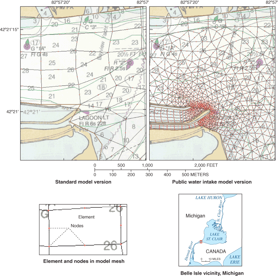
Figure 12. Standard and public water intake model grid topologies near Belle Isle, Michigan.
Particle tracking is used to describe the effects of molecular and turbulent diffusion on the dispersion of constituents with time. When computed in reverse time, the results may be used to identify areas upstream from points of withdrawal that are likely to contribute flow. When computed in forward time, the results may be used to identify potentially sensitive areas downstream from a point discharge.
The decision to compute in reverse or forward time only affects the signs of the velocity field simulated by the hydrodynamic model. In particular, the signs of the simulated velocity field are reversed when particle tracking in reverse time; no changes occur to the simulated velocity field when computing in forward time. The mathematics describing diffusion do not change as a function of the direction of particle tracking.
As part of the MDEQ Source Assessment Program, results of hydrodynamic simulations describing advection were combined with results of particle tracking describing diffusion to identify source areas to PWIs. This report illustrates the techniques used in the source water assessments by analyses of arbitrary locations on St. Clair River and Lake St. Clair. A simplified algorithmic description of mathematical techniques for modeling diffusion is presented to provide a basic understanding of the approach. Those interested in additional details may wish to consult Fischer and others (1979).
Hydrodynamic simulation describes the average movement (advection) of water in two dimensions for specified waterway geometry, hydraulic characteristics, and boundary conditions. In addition to advection, constituents introduced into the waterway are transported by diffusion. Diffusion occurs on the atomic scale as molecular diffusion, and on much larger scales of motion, associated with the range of eddy sizes present in the waterway, as turbulent diffusion.
Molecular diffusion is not of great consequence as a transport phenomenon in natural waterways, but is primarily significant on the scale of chemical and biological reactions. The mathematics describing molecular diffusion, however, provide a basis for the more general problem of describing diffusion transport. Fischer and others (1979) develop the mathematics for characterizing molecular and turbulent diffusion by use of statistical methods.
Molecular diffusion occurs as the result of a large number of random collisions among molecules. The collision rate depends on the viscosity and density of the fluid, and the size of the particles. Because of the large number of random collisions, a particle quickly loses the memory of its initial position and its motion becomes a random path, which is described as a random walk process (Fischer and others, 1979). If the motion of a single particle has a random component, the movement of a large number of particles may be described statistically.
In this report, the advective-diffusive movement of hypothetical particles in the waterway is approximated by combining the two-dimensional advective movement simulated by the hydrodynamic model with a two-dimensional random walk process that results from the cumulative effects of random perturbations of particle locations from the Gaussian or normal distribution. To describe source areas for public water supplies rather than destinations of point discharges, the signs of simulated velocities are reversed so that positive time increments in the simulation correspond to negative time in the waterway.
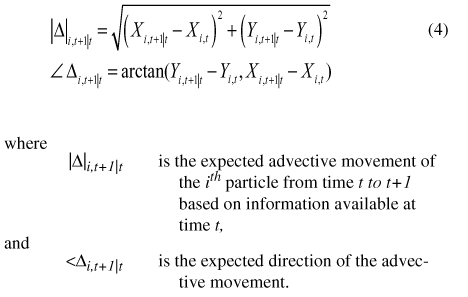
To initiate particle tracking, the location of a public water intake or other arbitrarily selected location is specified by its Easting (Xo) and Northing (Yo) coordinates. The number of hypothetical particles for tracking analyses also is specified, by say upper case I, and indexed from 1 to I by the lower case i. Initially, Xi,0 = Xo and Yi,o = Yo for all i. Finally, the length of the particle-tracking simulation T is specified along with the computation time step interval Δt. For compactness of notation, t +1xΔt is written as t+1, beginning at t=0.
The rate of particle diffusion is controlled by flow velocities and by the specified magnitude of two parameters: DiffL, for longitudinal (in the principal direction of flow) diffusion, and DiffT, for transverse (across the principal flow direction) diffusion. These two parameters specify the variance of the random variates returned from the normal distribution at each time step, as a function of the advective movement. For example, a value of 1/12 sets the variance of random movements to 1/12 of particle movement computed by advection. Given that longitudinal velocities tend to be larger than transverse velocities in rivers, longitudinal dispersion would tend to be larger than transverse dispersion even if DiffL were set equal to DiffT.
Solution files from hydrodynamic simulations provide a basis for determining advective movement in particle-tracking analyses. Solution files contain the simulated velocities and water levels at all nodes in the finite element mesh. Then, given a particle i location at time t, {Xi,t, Yi,t}, quadratic interpolation of the nodal velocities is used to approximate advective velocities across the corresponding element. These interpolated velocities are used with Δt to determine the advective movement and position for the next time step. The predicted position of the ith particle at the next time step, based only on the advective movement, is denoted {Xi,t+1|t, Yi,t+1|t}. The expected advective movement is then computed as:
The random longitudinal displacement of the ith particle at time t is:
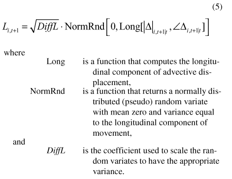
Similarly, the transverse component of the perturbation is

where Tran is a function that computes the transverse component of advective displacement.
Finally, particle locations are determined that include both advective and diffusive components as:
where analogous to the functions Long and Tran, East and Nrth are functions that return the Easting and Northing components from the logitudinal and transverse components.
The process continues as above for all particles and all time steps to complete the particle tracking simulation. The collection of all particle locations at one or more time steps shows the diffusion characteristics. The collection of all particle locations for an individual particle over time shows a particle track.
A generalized particle tracking code (ParTrac, v. 1.0) was developed in FORTRAN by the U.S. Army Corps of Engineers at the Waterway Experiment Station in Vicksburg, Mississippi (Ronald E. Heath, USACE WES, written commun., September 30, 2003). The program reads hydrodynamic solution files generated by RMA2 and creates output files of particle tracks that can be displayed within SMS. Currently, the program allows the specification of only one initial particle location, although up to 10,000 uniquely identifiable particles may be positioned at that location. The particle-tracking code is maintained in the public domain.
ParTrac generates a sequence of normally distributed pseudo-random numbers to simulate the effects of diffusion. Although the pseudo-random number sequence appears random, it is generated by a deterministic algorithm. The random number seed determines the uniqueness of the sequence returned by the algorithm. The seed may be specified by the user to ensure reproducibility, or assigned automatically, for example, based on the computer clock time, to provide alternative realizations of the number sequence.
The open-source code for ParTrac, which will remain in the public domain, was developed as part of the Source Water Assessment Program, which was initiated by MDEQ and supported by Detroit Water and Sewerage Department and the American Water Works Association Research Foundation. Documentation for the particle tracking code, which will provide a detailed description of the approach, input requirements, and output results is in preparation (John Koschik, USACE Detroit District, written commun., December 31, 2003).
Steady-state hydrodynamic simulations were developed by use of the PWI version of the Source Water Assessment Model of the St. Clair-Detroit River Waterway. The simulations describe the effects of mesh geometry and boundary conditions on local velocities in the waterway. A set of boundary condition scenarios were developed to help assess source areas to public water intakes or other arbitrarily selected locations.
Velocities computed at model nodes are determined by the mesh geometry and topology, and by boundary condition specifications. In areas where flow is obstructed by islands, for example, simulated flow fields detail the complex flow patterns that result. In addition, figure 13 illustrates the variation in the resolution of the velocity field with the density of nodes. Quadratic interpolation is used to estimate the velocity distribution across elements based on velocities computed at nodes. This interpolated velocity describes the advective flow used in particle tracking analyses.
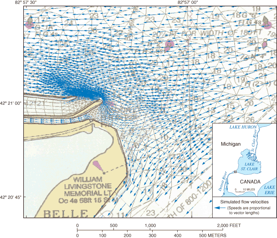
Figure 13. Advective velocities simulated at model nodes near Belle Isle, Michigan.
Boundary conditions specify external flows, water levels, and wind conditions to the waterway. The primary flow specification is at the head of St. Clair River, which accounts for the outflow of Lake Huron and more than 90 percent of the flow through the waterway. Additional minor-flow specifications include those for intervening tributaries, such as Black River on St. Clair River, Clinton River on Lake St. Clair, River Rouge on Detroit River, and net atmospheric and ground-water inputs to Lake St. Clair. Finally, flow specifications were used to describe withdrawals at public water intakes. Water levels were specified only at the water-level gaging station at Bar Point, Ontario, near the mouth of Detroit River. Wind boundary conditions for the entire waterway were based on measured conditions at station LSCM4 on Lake St. Clair, which is operated as by the National Data Buoy Center (http://www.ndbc.noaa.gov/station_page.php?station=lscm4) on August 12, 2004.
The range of flow, water level, and wind boundary conditions affecting the waterway is extensive. Developing a limited number of scenarios to span this range of interrelated conditions is problematic. In this report, only flows at the head of St. Clair River, water levels at the mouth of Detroit River, and winds were varied. Specifically, flow scenarios were utilized to describe the systematic variation in hydrodynamics with flows at the head of St. Clair River and associated water levels near the mouth of Detroit River for average wind conditions. Similarly, wind scenarios were utilized to describe the effects of varying wind conditions on water levels and velocities using average inflow and water level conditions. All other boundary conditions for both types of scenarios were maintained at constant values. In particular, average flow rates from intervening tributaries (Holtschlag and Koschik, 2001), and average withdrawal rates at public water intakes were constant for all scenarios.
Primary boundary conditions for flow scenarios include flows (discharges) at the head of St. Clair River near Port Huron, Michigan, and water levels at the Bar Point, Ontario, gaging station operated by the Canadian Water Survey. Flow can be measured directly at the head of St. Clair River in less than one hour by use of ADCP surveys. By themselves, however, these direct flow measurements do not provide a mechanism for computing continuous flow information. This information is needed for the development of flow scenarios, which require statistics from continuous flow data.
Efforts have been made by various federal agencies to provide a means of computing continuous flow data. Specifically, data from periodic direct-flow measurements are related to continuous measurements of water levels by use of a stage-fall-discharge rating. In such a relation, concurrent values of stage (water levels), for example at Fort Gratiot (NOAA station 9014098), and the fall, or difference in water levels between Fort Gratiot and the Mouth of Black River (NOAA station 9014090), are used to estimate direct measurements of discharge (flow) on upper St. Clair River. Although resulting stage-fall-discharge ratings do provide a continuous estimate of flow, there is substantial uncertainty in the estimated flows, perhaps exceeding 10 percent. The uncertainty has led to the development of different ratings among different U.S. and Canadian federal agencies, and restrictions on the application of the rating to estimating monthly mean flows. Estimation of flows over hourly or shorter intervals is problematic and remains a significant source of uncertainty on the accuracy of water budget and hydrodynamic simulations. Continuous velocity measurements near the head of St. Clair River, such as those obtainable with a fixed-station horizontal ADCP, may help improve the accuracy of continuous flow data.
The Coordinating Committee for Great Lakes Basic Hydraulic and Hydrologic Data meets periodically to review estimates of monthly mean flow, resolve discrepancies in flow estimates among federal agencies, and publish monthly mean flows for the Great Lakes. This binational committee reports directly to the International Joint Commission (IJC). The IJC is an independent binational organization established by the Boundary Waters Treaty of 1909. Its purpose is to help prevent and resolve disputes relating to the use and quality of boundary waters and to advise Canada and the United States on related questions. Finalized monthly hydrologic data from 1860 to 1990 have been compiled by Hunter and Croley (1993).
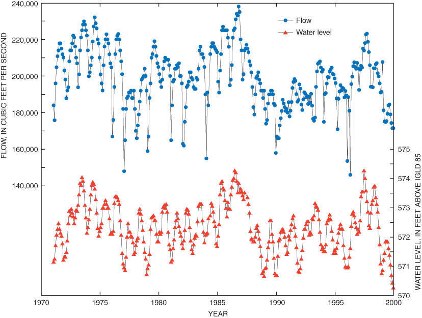
In this report, flows of St. Clair River were characterized based on monthly mean values from 1971 to 1999. Corresponding monthly mean water levels are published by the Canadian Water Survey for Bar Point, Ontario. A seasonal pattern and correlation is evident in flow and water-level data (fig. 14).
The range of monthly mean flows on St. Clair River may be characterized by a flow duration curve. This curve, either derived empirically from the monthly flow values, or approximated theoretically by a fitted cumulative normal distribution function, describes the probability that flow of a particular magnitude will be equaled or exceeded. Thus, for example, based on data for St. Clair River from 1970 to 1999, there is a 50 percent chance that flows will exceed 197,800 ft3/s (fig. 15). The continuous flow duration characteristics of St. Clair River are represented in 10 flow scenarios by use of the midpoint of the 10 flow deciles (table 3). Monthly mean flows of St. Clair River were related to monthly mean water levels at Bar Point, Ontario (fig. 16). A linear regression equation was developed to approximate this relation. This equation was used to compute expected water levels for the midpoint of each flow decile used in flow scenarios (table 3).
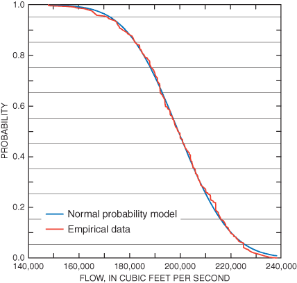
Figure 15. Monthly flow duration characteristics of St. Clair River.
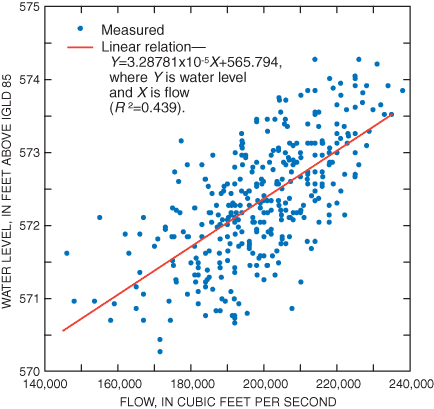
Table 3. Selected flow magnitudes on St. Clair River and water levels at Bar Point, Ontario. .
| Scenario identifier | Exceedance probability | Flow magnitude, in cubic feet per second | Expected water level at Bar Point, Ontario, in feet (IGLD 1985) | Wind speed, in miles per hour | Wind direction (blowing toward), counter clockwise from zero degrees east | Estimated probability |
|---|---|---|---|---|---|---|
| St. Clair and Detroit River Connecting Channel Scenarios | ||||||
| CC01 | 0.95 | 171,492 | 571.432 | 3.374 | 25.4 | 0.1000 |
| CC02 | .85 | 182,294 | 571.787 | 3.374 | 25.4 | .1000 |
| CC03 | .75 | 188,884 | 572.004 | 3.374 | 25.4 | .1000 |
| CC04 | .65 | 192,334 | 572.118 | 3.374 | 25.4 | .1000 |
| CC05 | .55 | 196,962 | 572.270 | 3.374 | 25.4 | .1000 |
| CC06 | .45 | 201,357 | 572.414 | 3.374 | 25.4 | .1000 |
| CC07 | .35 | 205,812 | 572.561 | 3.374 | 25.4 | .1000 |
| CC08 | .25 | 211,559 | 572.750 | 3.374 | 25.4 | .1000 |
| CC09 | .15 | 216,260 | 572.904 | 3.374 | 25.4 | .1000 |
| CC10 | .05 | 224,975 | 573.191 | 3.374 | 25.4 | .1000 |
Primary boundary conditions for wind scenarios were based on statistics from wind measurements at the weather stations on Lake St. Clair. The accuracy of these hydrodynamic simulations is affected by the wind drag formula and corresponding wind drag coefficients specified in the model. Drifting buoys were deployed and ADCP measurements of velocity were obtained in Lake St. Clair (Holtschlag, Syed, and Kennedy, 2002) to help confirm the adequacy of the original wind formula used in RMA2 (Donnell and others, 2003).
Specifically, buoy deployment data were compared with the movement of hypothetical drogues. Like particles, the initial position of drogues can be specified explicitly and tracked through time within SMS. Unlike particles, drogues move only with advection; they do not contain a random component. Results indicated that buoys appeared to move in the direction that the wind was blowing more than the drogues indicated. These results were interpreted as indicating that wind acting directly on exposed buoy surfaces pushed the buoys with the wind more effectively than it drove the depth-average water velocities. Given the difficulty of adjusting buoy movements for the direct effects of wind, the buoy deployment data were considered inconclusive in verifying or refuting the default wind drag coefficients. Current-velocity data from one or more fixed-station buoys deployed on Lake St. Clair are needed to help verify and confirm wind drag coefficients. For this analysis, the original RMA2 wind formula and coefficients were used for simulations.
A weather station (LSCM4) was established at the St. Clair River Light on Lake St. Clair as part of the Source Water Assessment Program. The station was created, and is operated and maintained, by the National Data Buoy Center (NDBC), which is part of the National Weather Service. At this station, wind speed and direction are measured 47.2 ft, air temperature is measured at 19.7 ft, and barametric pressure is measured at 1.3 ft above the average water surface at 10-minute intervals. NDBC reports the direction that the wind is coming from, in degrees clockwise from true north, and wind speed, in meters per second, averaged over an eight-minute interval. Both historical and real-time data are available through the internet (http://www.ndbc.noaa.gov/station_page.php?station=lscm4).
In this report, wind characteristics are described on the basis of LSCM4 data obtained from November 8, 2001, the first available data, to October 23, 2003, when this information was processed. Vector averages of data at 10-minute intervals were used to compute daily mean values, which were displayed in a wind chart (fig. 17).
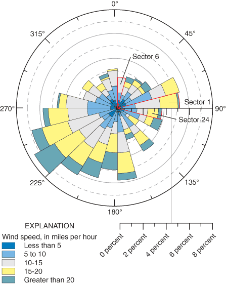
Figure 17. Winds characteristics on Lake St. Clair by sector.
In this wind chart, wind directions were arbitrarily divided into 24 sectors each having an angular width of 15 degrees. Sectors are numbered counterclockwise, starting at the sector from 90 to 75 degrees east of north. Within each sector, annuli describe the percentage of time daily mean wind speeds were within specified 5-mile-per-hour intervals. Average wind speeds and directions were computed for each sector. Average wind directions were transformed following the convention for input into RMA2, which describes the direction that winds are blowing toward and references angles counterclockwise from the positive x axis (zero degrees east) and listed in table 4. Thus, a wind reported by NDBC from the southeast, at 130 degrees, for example, would be described as a wind blowing toward the northwest at 140 degrees for input into RMA2. To complete the boundary condition specification for the 24 wind scenarios, flow at St. Clair River was specified as 199,170 ft3/s, and the water level at Bar Point, Ontario was specified as 572.342 ft IGLD 85.
Table 4. Wind characteristics at the weather station on Lake St. Clair.
| Sector | Number of days | Speed (miles per hour) | Average direction, measured counter clockwise from east | Estimated probability |
|---|---|---|---|---|
| 1 | 35 | 12.109 | 189.89 | 0.0491 |
| 2 | 36 | 10.310 | 201.56 | 0.0505 |
| 3 | 22 | 11.933 | 216.00 | 0.0309 |
| 4 | 20 | 9.851 | 232.49 | 0.0281 |
| 5 | 19 | 11.706 | 245.92 | 0.0266 |
| 6 | 18 | 8.259 | 260.15 | 0.0252 |
| 7 | 23 | 9.407 | 277.07 | 0.0323 |
| 8 | 21 | 10.300 | 292.70 | 0.0295 |
| 9 | 17 | 9.380 | 309.02 | 0.0238 |
| 10 | 23 | 8.989 | 323.76 | 0.0323 |
| 11 | 20 | 8.046 | 336.27 | 0.0281 |
| 12 | 34 | 10.297 | 353.60 | 0.0477 |
| 13 | 42 | 12.069 | 9.44 | 0.0589 |
| 14 | 50 | 14.191 | 23.95 | 0.0701 |
| 15 | 54 | 15.215 | 37.25 | 0.0757 |
| 16 | 45 | 13.239 | 52.48 | 0.0631 |
| 17 | 42 | 14.571 | 66.38 | 0.0589 |
| 18 | 36 | 15.902 | 81.88 | 0.0505 |
| 19 | 42 | 13.237 | 96.86 | 0.0589 |
| 20 | 19 | 13.477 | 115.58 | 0.0266 |
| 21 | 29 | 12.287 | 125.91 | 0.0407 |
| 22 | 15 | 12.260 | 144.12 | 0.0210 |
| 23 | 26 | 12.061 | 157.76 | 0.0365 |
| 24 | 25 | 11.985 | 172.24 | 0.0351 |
Ten flow scenarios and 24 wind scenarios were developed to characterize velocity distributions on the waterway. Applying every possible combination of these scenarios would require 240 steady-state simulations. Evaluating the results of 240 hydrodynamic simulations at 13 public water intakes on the United States side of the waterway would require 3,120 particle-tracking analyses. This type of combinational approach would be computationally prohibitive.
As a possible alternative, applying different types of scenarios to different parts of the waterway was evaluated. Evaluation of this alternative was based on the spatial sensitivity of hydrodynamics to the type of boundary condition. In this evaluation, changes in water speed at individual nodes were used in the assessment of sensitivity. Changes in water speed were computed for the maximum differences of both flow and wind scenarios.
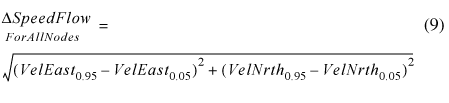
In particular, flow scenarios at the 5 percent and 95 percent exceedance intervals were selected as the two scenarios likely to have the greatest difference between simulated water velocities. Easting and northing velocity components were computed at all nodes for both flow scenarios and identified as VelEast0.05, VelNrth0.05, VelEast0.95, and VelNrth0.95, respectively. Changes in water speeds were computed as:
Similarly, wind scenarios for winds in sectors 2 and 14 were selected to represent the most dissimilar effects of winds on flow velocities, because these two sectors had the greatest difference in wind magnitudes and directions. Again, changes in water speeds between scenarios were computed as:
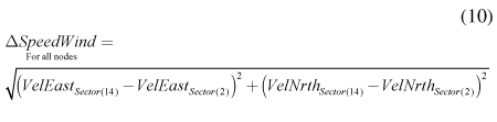
Finally, a measure of relative sensitivity was computed as the Log10 ratio of speed changes as:
The bimodal distribution of WindFlow values indicated by the histogram is (fig. 18) is interpreted as representing two populations of sensitivities, best separated at the midpoint of the distribution. Nodes with generally lower values of WindFlow are interpreted as a population where flow scenarios have the dominant effect on local velocities; whereas nodes with generally higher values of WindFlow are from a population where wind scenarios dominant local velocities. Using the midpoint of the distribution to separate the populations, a map of the waterway indicates that the flow-dominated nodes generally occur within the St. Clair and Detroit Rivers, whereas the wind-dominated nodes generally occur within Lake St. Clair.
Figure 18. Areas of wind and flow dominated effects on the St. Clair-Detroit River Waterway.
This result supports the use of flow scenarios to identify source areas to public water intakes on the St. Clair and Detroit Rivers, and wind scenarios to identify source areas on Lake St. Clair. This conclusion also is supported by the fact that flow depths on the St. Clair and Detroit Rivers average about twice the depths of flow on Lake St. Clair, making surface winds more influential on depth-averaged flows.
Particle tracking analyses are presented for St. Clair River and Lake St. Clair to illustrate the techniques used in the source water assessment of public water intakes. The flow dominated and wind dominated particle-tracking analyses share some common features, but have distinct differences as well. Both analyses were based on steady-state velocities simulated by the public water intake version of the St. Clair-Detroit River Model developed for the Source Water Assessment Program. All particle tracking was done in reverse time (upstream direction). Because of differences between sensitivities to boundary conditions, St. Clair River delineations were based on the ten flow-based scenarios; while Lake St. Clair delineations were based on 24 wind-based scenarios. Delineations for both St. Clair River and Lake St. Clair involved 10,000 hypothetical particles. In the analysis of St. Clair River, 1,000 particles were used in each of the 10 flow scenarios, corresponding to the equal probabilities of the selected flow conditions. In contrast, different numbers of particles were included in the wind-based scenarios; the distribution of particles among scenarios, however, also was based on the probability of the wind conditions. In both St. Clair River and Lake St. Clair analyses, the diffusion parameters DiffL and DiffT were set equal to 1/12. Given that flow velocities on St. Clair River commonly exceed 3.0 ft/s, while flow velocities on Lake St. Clair commonly are less than 0.3 ft/s, the magnitudes of random perturbations simulating diffusion on St. Clair River were greater than those simulating diffusion on Lake St. Clair.
Techniques for identifying source areas in flow-dominated areas of the St. Clair-Detroit River Waterway are illustrated by particle tracking results for upper St. Clair River near Port Huron, Michigan. Upper St. Clair River has high flow velocities and significant channel curvature that gives rise to secondary circulation patterns. Drifting buoy deployments on upper St. Clair River (Holtschlag and Aichele, 2001) indicate that upper waters on the Canadian side of the waterway cross to the U.S. side as flow passes from the Blue Water Bridge downstream to Black River. Depth-averaged velocities simulated by the model cannot reveal this tendency. Any changes in velocities with depth through the water column cannot be represented by a two dimensional depth-averaged model. A three-dimensional hydrodynamic model and particle tracking code is needed for these areas. Two-dimensional flow simulations, however, currently provide the basis for source area delineations of public water intakes on the St. Clair-Detroit River Waterway.
Particle tracks were computed based on hydrodynamic simulation results from 10 flow scenarios, each simulation including 1,000 particles. Particles were propagated through the waterway at 5-second time-step intervals for a period of up to 2 hours. Figure 19 shows the distribution of particle locations for each flow decile at 0.5-hour intervals. Results indicate that advective movements dominate diffusive effects in this reach as the differences among particle distributions between flow-scenarios becomes more apparent with the duration of the simulation.
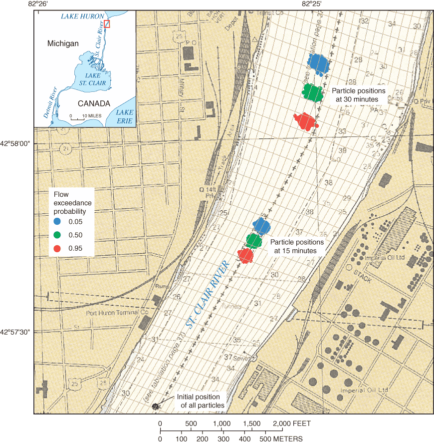
Figure 19. Particle tracking results on St. Clair River near Port Huron, Michigan.
Confirmation of the computed particle distribution results with field data is problematic. In an effort to provide a check on the plausibility of particle tracking results, however, experiments were conducted using drifting buoys equipped with GPS (Global Positioning System) receivers on St. Clair River (Holtschlag and Aichele, 2001), and Detroit River (Holtschlag and Aichele, 2002). According to Fischer and others (1979), "Tracking drogues" (buoys) "is very tedious and gives distressing little data in relation to costs." Although GPS equipment greatly improves the efficiency of buoy deployments, it was not possible to conduct enough deployments throughout the waterway to provide sufficient evidence that DiffL and DiffT differed from a value of 1/12, which is the default parameter values in ParTrac 1.0. Limited comparisons between the changes in the distribution of clustered buoys and changes in the distribution of computed particles with time, however, indicated general similarities. Thus, limited field data from buoy deployments confirms the plausibility of particle tracking results on rivers.
Although wind conditions are unlikely to remain constant for extended periods, particle movements in Lake St. Clair were simulated for a 3-day period to illustrate the sensitivity of source areas to wind direction in L'anse Creuse Bay (figs. 20-23). Particle positions were computed at 1-minute intervals and output at 5-minute intervals. Particle paths were based on wind-dominated scenarios described previously. Given the duration of the simulation, individual particle locations could not be readily shown. Results indicate that source areas can originate from any direction, as determined by the wind direction. Particle tracks of actual constituents would be much more variable because of the variability in wind velocities. Source areas might best be delineated by use of a curve that envelops all particle paths.
Rotational circulation patterns in L'anse Creuse Bay of Lake St. Clair may cause source areas and sink areas, such as public water intakes, to seem coincident. Rather, this implies that any constituent discharge near a PWI may periodically reoccur at the intake under the appropriate wind conditions.
A two-dimensional hydrodynamic model of the St. Clair-Detroit River Waterway has been developed, calibrated, and refined to identify source areas to PWIs. Additional instrumentation and further model development would improve the utility and accuracy of the model for continuous simulation needed for real-time flow information at hourly (or shorter time) intervals. This flow information is critical for characterizing the water budget of the St. Clair-Detroit River Waterway, for protecting drinking water supplies, and for responding to contaminant spills and discharges in real time.
Substantial simulation uncertainty results from uncertainty in the flow boundary specification at the head of St. Clair River, which accounts for about 95 percent of the flow through the waterway. Various federal agencies in the United States and Canada have developed alternative stage-fall-discharge relations to compute flow based on the continuously monitored water-level data. Uncertainties and conflicting results obtained from these mathematical relations have limited estimation intervals to monthly mean flows, which involve substantial delays in publication associated with binational reconciliation efforts.
Computation of waterway flows at hourly intervals will require the development of more accurate means for determining the dominant flow boundary. Installation of a horizontal acoustic Doppler current profiler (H-ADCP) in upper St. Clair River would provide a continuously updated set of index velocity measurements extending a significant distance across the river. This velocity data would be a critical complement to an existing network of NOAA water-level monitoring stations and routine ADCP flow measurements by the USACE. Velocity, water level, and flow data would provide the basis for developing an improved mathematical relation for computing hourly inflows.
Wind is the primary mechanism determining circulation patterns in Lake St. Clair. Continued operation and maintenance of the National Data Buoy Center weather station at the St. Clair Light on Lake St. Clair (Station LSCM4) would provide boundary condition data needed for flow simulation. Addition of a tethered buoy for monitoring water currents at various points on Lake St. Clair would provide data needed to confirm, and modify if necessary, the wind drag formula and associated coefficients.
Upper St. Clair River, between the head of St. Clair River and the mouth of Black River, is characterized by high flow velocities, which may exceed 5 ft/s, and significant channel curvature. This reach, which includes a public water intake for the city of Port Huron, Michigan, has flow conditions that commonly give rise to large secondary recirculation patterns. Flow simulation results indicate that depth-averaged velocities simply parallel the curvature in the channel shoreline. In contrast, drifting buoy deployments (Holtschlag and Aichele, 2001) indicate that surface velocities tend to drift across the river toward the outside of the channel curvature. To compensate, lower waters are thought to flow toward the inside of the channel curvature. Whatever the reason for the discrepancies between flow simulation and drifting buoy results, failure of flow simulations to account for complex flow structures or significant velocity variations with depth would result in misidentification of source areas to public water intakes for the city of Port Huron, Michigan.
A three-dimensional hydrodynamic model would provide a basis for simulating complex flow structures in the St. Clair-Detroit River Waterway. This information would help resolve discrepancies between field measurements of velocity patterns and simulated velocity characteristics. Further, an improved understanding of the hydrodynamics of the waterway would provide information needed to better assess and predict sediment and contaminant transport. Development of the two-dimensional model has provided information on channel bathymetry, geometry, flow partitioning around numerous islands and dikes in the waterway, water level information, and velocity measurements to facilitate the development and calibration of a three-dimensional model. Finally, limited information was available for assessing the adequacy or refining the accuracy of diffusion coefficients DiffL and DiffT. Thus, the understanding of diffusion processes on the St. Clair-Detroit River Waterway is limited.
A two-dimensional hydrodynamic model of the St. Clair-Detroit River (Holtschlag and Koschik, 2002) was recalibrated and refined to identify source areas to public water intakes. RMA2 (Donnell and others, 2003) was the hydrodynamic code used for flow simulations. SMS (Environmental Modeling Research Laboratory, 2003) was used to pre- and post-process model input and output files. Using the initial finite-element mesh design from Holtschlag and Koschik (2002), the model was recalibrated by approximating the systematic change in channel roughness as a nonlinear function of flow depth, and by estimating the Peclet number used to assign eddy viscosity characteristics to model elements. Recalibration added point-velocity data obtained from acoustic Doppler current profiler surveys of St. Clair and Detroit Rivers, to data on flow and water levels used in the previous calibration. Parameters were estimated by use of a nonlinear regression technique developed by Hill (1998) and implemented within the computer program UCODE by Poeter and Hill (1998). Overall, recalibration resulted in a slight improvement in model accuracy; flows were estimated with marginally less accuracy, while water levels and velocities were estimated with somewhat greater accuracy. Calibration results document the accuracy of simulated flows, water levels, and velocities. The recalibrated model with the initial mesh design supersedes the initial model, and is now considered the standard version of the St. Clair-Detroit River Waterway model developed for source-water assessments.
A public water intake version of the model was developed by refining the finite element mesh of the standard version. Refinements were used to improve the resolution of flow velocities near public water intakes. Refinements generally resulted from subdivisions of existing elements into four (sub) elements; additional nodes and elements were added to detail hydraulic features near public water intakes that were omitted in the standard version. Refinements increased the number of nodes from 42,936 in the standard version to 90,386 nodes in the public water intake version, and caused a commensurate increase in model execution times and memory requirements. The public water intake version of the model was used to develop flow simulations to identify source areas to public water intakes.
Two types of scenarios were developed for simulation analysis. Ten flow scenarios describe the range in expected flow conditions by specifying the inflow at the head of St. Clair River and a corresponding water level at the mouth of Detroit River. Inflows were specified at the midpoint of the deciles of the monthly mean flow distribution on St. Clair River. Corresponding water levels at the mouth of Detroit River were based on a regression equation describing the relation between monthly mean flows on St. Clair River and monthly mean water levels near the mouth of Detroit River. Flow scenarios were based on average wind speeds and inflows from local tributaries. Twenty-four wind scenarios describe the expected range of wind conditions based on wind data obtained on Lake St. Clair. Each scenario represents the average wind speed in 24 compass sectors, each having an angular width of 15 degrees. Sensitivity analysis indicated that the St. Clair and Detroit Rivers were sensitive to flow scenarios, and Lake St. Clair was sensitive to wind scenarios. To illustrate the technique for source area identification, 10 flow scenarios were used to simulate advection on St. Clair River, and 24 wind scenarios were used to simulate advection on Lake St. Clair.
ParTrac, a particle tracking code developed by the USACE WES, was used to describe the expected movement of hypothetical particles by combining advection described by hydrodynamic flow simulations with molecular and turbulent diffusion described by a two-dimensional random-walk process. Particle tracking was simulated in reverse time by changing the signs of simulated velocity components. To illustrate the techniques used for source water assessments of public water intakes, particles were placed at arbitrarily selected destinations on St. Clair River and Lake St. Clair and tracked backward in time to their respective source areas. Results show the sensitivity of particle tracking to flow conditions on St. Clair River and wind conditions on Lake St. Clair.
Current model limitations include: (1) inadequate inflow information at the head of St. Clair River for accurate model simulations; (2) uncertainty in the effects of wind on circulation in Lake St. Clair; (3) inconsistencies between drifting buoy tracks and simulated velocities in upper St. Clair River; and (4) uncertainties in the parameterization of diffusion processes. Model enhancements needed to address current model limitations include: (1) installation of a continuous horizontal acoustic Doppler current profiler in upper St. Clair River to provide more precise inflow information; (2) continuous monitoring of point velocities in Lake St. Clair to provide a basis for quantifying wind effects; (3) development of a three-dimensional version of the flow model to resolve complex flow patterns; and (4) further study on the diffusion characteristics of the waterway.
A binational technical workgroup provided suggestions, recommendations, and data that facilitated model implementation. Workgroup members and associates included Brad Brogren, Michigan Department of Environmental Quality, Source Water Assessment Program; Gang Song and Bahi Habib, Detroit Water and Sewerage Department; and Syed Moin and Aaron Thompson, Environment Canada, Canada Centre for Inland Waters. Christopher Rayburn, Research Management Director, American Water Works Association Research Foundation, Ramesh Kashinkunti, Senior Engineer, Department of Water Works, City of Cincinnati, Ohio, and Scott Wells, Professor and Chair of Environmental Engineering, Portland State University, also provided technical direction and review.
Cressie, N.A.C., 1991, Statistics for spatial data: New York, John Wiley, 900 p.
Donnell B.P., Letter, J.V., Jr., McAnally, W.H., and Thomas, W.A., 2003, Users guide to RMA2-WES Version 4.5: U.S. Army Corps of Engineers Waterway Experiment Station, Vicksburg, Miss., 264 p. [http://chl.wes.army.mil/software/tabs/docs.htp, October 14, 2003.].
Environmental Modeling Research Laboratory, 2003, SMS Surface-Water Modeling System Reference Manual (version 7): Environmental Modeling Systems, Inc., Provo, Utah, 342 p.
Fischer, H.B., List, E.J., Koh, R.C.Y., Imberger, Jörg, and Brooks, N.H., 1979, Mixing in inland and coastal waters: New York, Academic Press, 483 p.
Hill, M.C., 1998, Methods and guidelines for effective model calibration: U.S. Geological Survey Water-Resources Investigations Report 98-4005, 90 p.
Holtschlag, D.J., and Aichele, S.A., 2001, Visualization of drifting buoy deployments on St. Clair River near Public Water Intakes - October 3-5, 2000, U.S. Geological Survey Open-File Report 01-17, http://mi.water.usgs.gov/splan2/sp08903/SCRIndex.html
Holtschlag, D.J., and Aichele, S.A., 2002, Visualization of Drifting Buoy Deployments on Upper Detroit River within the Great Lakes Waterway from August 28-30, 2001, U.S. Geological Survey Open-File Report 02-1, http://mi.water.usgs.gov/pubs/OF/OF02-1/.
Holtschlag, D.J., and Koschik, J.A., 2001, Steady-state flow distribution and monthly flow duration in selected branches of St. Clair and Detroit Rivers, two connecting channels of the Great Lakes: U.S. Geological Survey Water Resources Investigations Report 01-4135, 45 p.
Holtschlag, D.J., and Koschik, J.A., 2002, A two-dimensional hydrodynamic model of the St. Clair-Detroit River Waterway in the Great Lakes Basin: U.S. Geological Survey Water Resources Investigations Report 01-4236, 63 p.
Holtschlag, D.J., and Koschik, J.A., 2003a, An acoustic Doppler current profiler survey of flow velocities in St. Clair River, a connecting channel of the Great Lakes, U.S. Geological Survey Open-File Report 03-119 [http://mi.water.usgs.gov/pubs/OF/OF03-119/].
Holtschlag, D.J., and Koschik, J.A., 2003b, An acoustic Doppler current profiler survey of flow velocities in Detroit River, a connecting channel of the Great Lakes, U.S. Geological Survey Open-File Report 03-219 [http://mi.water.usgs.gov/pubs/OF/OF03-219/].
Holtschlag, D.J., Syed, A.U., and Kennedy, G.W., 2002, Visualization of a drifting buoy deployment on Lake St. Clair within the Great Lakes Waterway from August 12-15, 2002, Date Posted: December 19, 2002, U.S. Geological Survey Open-File Report 02-482 (http://mi.water.usgs.gov/pubs/OF/OF02-482/DriftingBuoyLSC.php)
Hunter, T.S., and Croley, II, T.E., 1993, Great Lakes Monthly Hydrologic Data, NOAA Data Report ERL GLERL, National Technical Information Service, Springfield, Virginia, 22161, 1993. (http://www.glerl.noaa.gov/data/arc/hydro/mnth-hydro.html, December 17, 2003). (Note: monthly mean flow data for St. Clair and Detroit Rivers has been updated to include data through 1999).
National Oceanic and Atmospheric Administration, 1999, Recreational chart 14853: Detroit River, Lake St. Clair, and St. Clair River: U.S. Department of Commerce, National Ocean Service, 1:15000 scale.
Poeter, E.P., and Hill, M.C., 1998, Documentation of UCODE, A computer code for universal inverse modeling: U.S. Geological Survey Water-Resources Investigations Report 98-4080, 116 p.
Schwab, D.J., Clites, A.H., Murthy, C.R., Sandall, J.E., Meadows, L.A., and Meadows, G.A., 1989, The effect of wind on transport and circulation in Lake St. Clair: Journal of Geophysical Research, v. 94, no. C4, April, p. 4947-4958.
Tsanis, I.K., Shen, Huihua, and Venkatesh, S., 1996, Water currents in the St. Clair and Detroit Rivers: Journal of Great Lakes Research, v. 22, no. 2, p. 213-223.
U.S. Army Corps of Engineers, 2001, Users Guide to GFGEN – Version 4.35, U.S. Army Corps of Engineers, Waterway Experiment Station-Hydraulic Laboratory, 53 p. [http://chl.wes.army.mil/software/tabs/docs/gfgen_05_2001.pdf, December 29, 2003].
Williamson, D.C., Scott R.D., and Lord, Stephen, 1997, Numerical modeling of the St. Clair/Detroit River system and seasonal variations in head loss, in Proceedings of the 1997 Canadian Coastal Conference, Guelph, Ontario, May 21-24, 1997, Canadian Coastal Science and Engineering Association, p. 176-184.
For more information concerning the research in this report, contact:
Jim Nicholas, District Chief
U.S. Geological Survey
6520 Mercantile Way, Suite 5
Lansing, MI 48911-5991
Document Accessibility: Adobe Systems Incorporated has information about PDFs and the visually impaired. This information provides tools to help make PDF files accessible. These tools convert Adobe PDF documents into HTML or ASCII text, which then can be read by a number of common screen-reading programs that synthesize text as audible speech. In addition, an accessible version of Acrobat Reader 6.0, which contains support for screen readers, is available. These tools and the accessible reader may be obtained free from Adobe at Adobe Access.
| AccessibilityFOIAPrivacyPolicies and Notices | |
 |
|