Scientific Investigations Report 2006–5226
In cooperation with the University of Wisconsin-Milwaukee
This report available for download (4,143 KB).
The appendix files are available for download as pdf (4,889 KB).
Abstract
Introduction
Purpose and Scope
Description of the Study Area
Note on Units of Measurement
Background and Application of Acoustic Doppler Current Profiler Technology
Acoustic
Doppler Current Profiler
Shear-Stress Estimation Method
Data-Collection Methods
Velocity-Profile Data
Water-Level Data
Data-Reduction Methods
Velocity-Profile Data
Water-Level Data
Results
Operable Unit 3 (OU–3)
Operable Unit 4 (OU–4)
Discussion
Effect of Boat Movement on Shear-Stress Estimates Made with the TKE Method
Differences in Roughness Length for OU–3 and OU–4
Comparison of Shear-Stress Parameters for
OU–3 and OU–4
Spatial Distribution of Estimated Shear Stress
Spatial and Temporal Variation in the Bottom Coefficient of Friction
Departures From the Ideal Log Velocity Profile
Repeatability of Shear-Stress Parameter Estimates
Summary and Conclusions
References Cited
Appendix: Velocity-Profile Plots for
OU–3 and OU–4
October 2004 Velocity Profiles (OU–3)
June 2003 Velocity Profiles (OU–4)
November 2003 Velocity Profiles (OU–4)
March 2004 Velocity Profiles (OU–4)
May 2004 Velocity Profiles (OU–4)
Figure 1. Map of the Lower Fox River study area, Wisconsin.
Figure 2. Diagram of the acoustic Doppler current meter transducer configuration.
Figure 3. Graph showing a typical velocity profile obtained using the acoustic Doppler current meter.
Figure 4. Map of acoustic Doppler current meter deployment sites with valid profiles within Operable Unit 3, Lower Fox River, Wis.
Figure 5. Graph showing recorded water surface elevations in Operable Unit 3, September and October 2004.
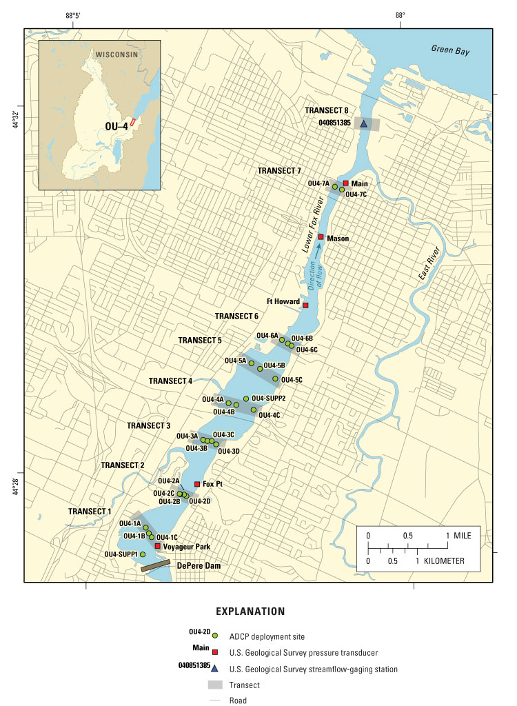
Figure 6. Map of acoustic Doppler current meter deployment sites with valid profiles within Operable Unit 4, Lower Fox River, Wis.
Figure 7. Graphs showing Example of measured water-level fluctuations at all measurement sites, Lower Fox River, Wis., November 5–7, 2003.
Figure 8. Graphs showing Log-profile (LP) and total-kinetic-energy (TKE) estimates of shear stress for various standard deviations in heading, Operable Unit 3, Lower Fox River, Wis.
Figure 9. Graphs showing estimated roughness lengths, OU–4, Lower Fox River, Wis.
Figure 10a. Map showing distribution of calculated shear stress during May 2005 sampling event, Operable Unit 4 (transects 1 through 3), Lower Fox River, Wis.
Figure 10b. Map showing distribution of calculated shear stress during May 2005 sampling event, Operable Unit 4 (transects 3 through 6), Lower Fox River, Wis.
Figure 11a. Map showing distribution of the bottom coefficient of friction calculated from November 2003 and March and May 2004 profiles, Operable Unit 4 (transects 1 through 3), Lower Fox River, Wis.
Figure 11b. Map showing distribution of the bottom coefficient of friction calculated from November 2003 and March and May 2004 profiles, Operable Unit 4 (transects 3 through 6), Lower Fox River, Wis.
Figure 12. Graphs showing variation in the bottom coefficient of friction with depth in Operable Unit 3, Lower Fox River, Wis.
Figure 13. Graphs showing variation in the bottom coefficient of friction with depth in Operable Unit 4, Lower Fox River, Wis.
Figure 14. Graphs showing example of a close-to-ideal velocity profile.
Figure 15. Graphs showing example of a velocity profile strongly influenced by the wind.
Figure 16. Graphs showing example of a velocity profile showing possible bedform influences.
Table 1. Calculated recurrence intervals for the Fox River at Appleton, Wis.
Table 2. Project acoustic Doppler current meter (ADCP) configuration.
Table 3. Summary statistics, Operable Unit 3 velocity profiles, October 2004.
Table 4. Summary of velocity profiles by water depth.
Table 5. Summary statistics, Operable Unit 4 velocity profiles, June 2003, Lower Fox River, Wis.
Table 6. Summary statistics, Operable Unit 4 velocity profiles, November 2003, Lower Fox River, Wis.
Table 7. Summary statistics, Operable Unit 4 velocity profiles, March 2004, Lower Fox River, Wis.
Table 8. Summary statistics, Operable Unit 4 velocity profiles, May 2004, Lower Fox River, Wis.
Table 9. Roughness lengths for all acoustic Doppler current meter deployment events, Lower Fox River, Wis.
Table 10. Vertically averaged velocity for all events, Lower Fox River, Wis.
Table 11. Shear stress by log-profile method, 10–20 percent of depth, for all events, Lower Fox River, Wis.
Table 12. Shear stress by turbulent-kinetic-energy method for all events, Lower Fox River, Wis.
Table 13. Shear stress by log-profile method, 6–10 percent of depth, for all events, Lower Fox River, Wis.
Table 14. Comparison of replicate shear-stress estimates by the log-profile method.
Table 15. Comparison of replicate shear-stress estimates by the turbulent kinetic energy method.
Table 16. Comparison of replicate roughness length estimates.
|
Multiply |
By |
To Obtain |
||||||||||||||||
Length |
||||||||||||||||||
| centimeter (cm) | inch (in.) | |||||||||||||||||
| millimeter (mm) | inch (in.) | |||||||||||||||||
| meter (m) | foot (ft) | |||||||||||||||||
| inch (in.) | centimeter (cm) | |||||||||||||||||
| inch (in.) | millimeter (mm) | |||||||||||||||||
| foot (ft) | meter (m) | |||||||||||||||||
| mile (mi) | kilometer (km) | |||||||||||||||||
Area |
||||||||||||||||||
| square centimeter (cm2) | square inch (ft2) | |||||||||||||||||
| square mile (mi2) | hectare (ha) | |||||||||||||||||
Volume |
||||||||||||||||||
| cubic centimeter (cm3) | cubic inch (in3) | |||||||||||||||||
| cubic yard (yd3) | cubic meter (m3) | |||||||||||||||||
Flow rate |
||||||||||||||||||
| centimeter per second (cm/s) | inch per second (in/s) | |||||||||||||||||
| foot per second (ft/s) | |
meter per second (m/s) | ||||||||||||||||
| meter per second (m/s) | foot per second (ft/s) | |||||||||||||||||
| meter per second squared (m/s2) | foot per second squared (ft/s2) | |||||||||||||||||
| mile per hour (mi/h) | kilometer per hour (km/h) | |||||||||||||||||
| cubic foot per second (ft3/s) | cubic meter per second (m3/s) | |||||||||||||||||
| gram (g) | ounce, avoirdupois (oz) | |||||||||||||||||
| kilogram (kg) | pound, avoirdupoi (lb) | |||||||||||||||||
| pound, avoirdupois (lb) | kilogram (kg) | |||||||||||||||||
| dyne per centimeter squared (dyn/cm2) | ounce per inch squared (oz/in2) | |||||||||||||||||
| pascal (Pa) | pound per square foot (lb/ft2) | |||||||||||||||||
| millibar (mbar) | pascal (Pa) | |||||||||||||||||
| pound per square foot (lb/ft2) |
kilopascal (kPa) | |||||||||||||||||
| pound per square inch (lb/in2) |
kilopascal (kPa) | |||||||||||||||||
| gram per cubic centimeter (g/cm3) | pound per cubic foot (lb/ft3) | |||||||||||||||||
| joule (J) |
kilowatthour (kWh) | |||||||||||||||||
Vertical elevation information is referenced to the North American Vertical Datum of 1988 (NAVD 88) or the International Great Lakes Datum of 1985 (IGLD 85). Conversion between NAVD 88 and IGLD 85 is site-specific. Near the mouth of the Lower Fox River, elevations relative to IGLD 85 may be approximated by subtracting 0.1271 m (0.4167 ft) from the NAVD 88 elevation. Frequency is reported as kilohertz (kHz). Absolute temperature is reported as degrees Kelvin (°K).
|
||||||||||||||||||
Turbulent shear stress in the boundary layer of a natural river system largely controls the deposition and resuspension of sediment, as well as the longevity and effectiveness of granular-material caps used to cover and isolate contaminated sediments. This report documents measurements and calculations made in order to estimate shear stress and shear velocity on the Lower Fox River, Wisconsin.
Velocity profiles were generated using an acoustic Doppler current profiler (ADCP) mounted on a moored vessel. This method of data collection yielded 158 velocity profiles on the Lower Fox River between June 2003 and November 2004. Of these profiles, 109 were classified as valid and were used to estimate the bottom shear stress and velocity using log-profile and turbulent kinetic energy methods. Estimated shear stress ranged from 0.09 to 10.8 dynes per centimeter squared. Estimated coefficients of friction ranged from 0.001 to 0.025.
This report describes both the field and data-analysis methods used to estimate shear-stress parameters for the Lower Fox River. Summaries of the estimated values for bottom shear stress, shear velocity, and coefficient of friction are presented. Confidence intervals about the shear-stress estimates are provided.
Between the mid-1970s and the early 1980s, an estimated 279,000 to 881,000 lbs of polychlorinated biphenyl (PCB) was discharged to the Lower Fox River in northeastern Wisconsin (Wisconsin Department of Natural Resources, 1999). PCB was released to the river primarily as a result of the recycling of carbonless copy paper. Lower Fox River sediments are currently believed to contain about 62,900 lbs of PCB, with a total contaminated sediment volume of 11.46 million cubic yards (RETEC Group, Inc., 2002).
A remedial investigation and feasibility study of the contaminated sediment deposits generated a range of possible cleanup options, which include combinations of dredging and capping of the various sediment deposits (RETEC Group, Inc., 2002). The remedial investigation considered the Lower Fox River in four discrete areas, known as operable units (OU). A detailed evaluation of alternatives (DEA) was generated as a supplement to the work done as part of the Fox River Superfund process (RETEC Group, Inc., 2003). The DEA notes that of the four operable units, three are suitable for remediation options that include capping—a process in which contaminated sediments are covered with a protective layer of clean granular material. The DEA report also notes a lack of directly measured current velocities within each of the operable units and suggests that additional hydrodynamic data would improve estimates of maximum current velocities (RETEC Group, Inc., 2003). Better hydrodynamic data would improve the basis of sediment-cap designs.
In summer 2003, the U.S. Geological Survey (USGS), in cooperation with the University of Wisconsin−Milwaukee, began a program of data collection and data analysis in the Lower Fox River. The primary objective of this program was to collect the velocity profile data needed to calculate streambed shear stress and roughness in areas of the Lower Fox River identified as potentially suitable for sediment capping (RETEC Group, Inc., 2003).
This report summarizes the methods and results of a data-collection and data-analysis program by the USGS on the Lower Fox River in 2003 and 2004 between the Little Rapids Dam and Green Bay, Wis. Two types of data were collected: water-velocity profiles and water-surface elevations. The data were analyzed to produce estimates of bottom roughness, shear velocity, and shear stress at the sediment-water interface. Water-elevation data obtained in this work were used to establish downstream boundary conditions for possible application of a hydrodynamic model.
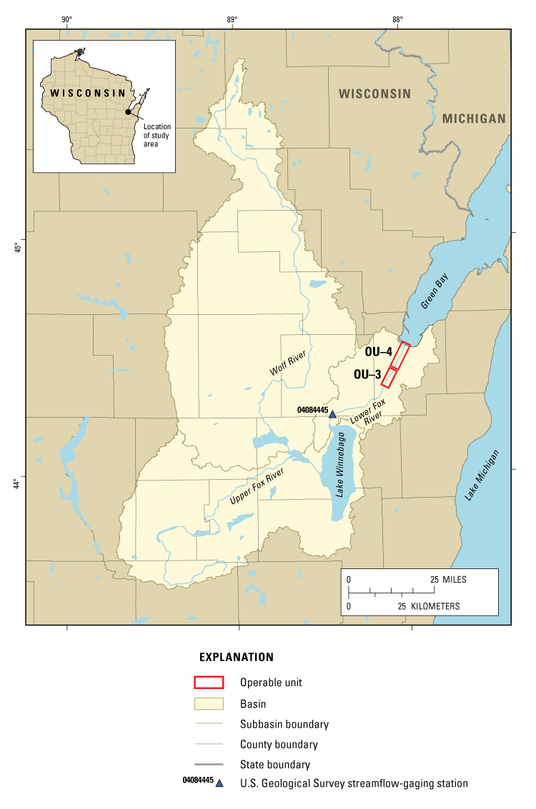
The Lower Fox River in northeastern Wisconsin (fig. 1) drains a basin with a total area of about 6,349 mi2. Of the total basin area, 89 percent drains into the 206-mi2 Lake Winnebago, from which flow enters the Lower Fox River proper. The Lower Fox River extends 39 mi from Lake Winnebago to Green Bay, Wis. Thirteen existing dams and one abandoned dam in this reach of river control river flows to balance ecological, public-safety, and power-generation needs (Wisconsin Department of Natural Resources, 2002).
Figure 1. Lower Fox River study area, Wisconsin.
The study area for the work described here encompassed the areas referred to in the remedial investigation/feasibility study as “OU–3” and “OU–4.” OU–3 extends downstream from the Little Rapids Dam to the DePere Dam, a distance of about 6 mi. OU–4 extends downstream about 7 mi from the DePere Dam to the confluence of the Lower Fox River and Green Bay (fig. 1).
The presence of Lake Winnebago and the dams on the Lower Fox River reduces the ratio between low and high flows, which results in the river being classified “stable” in terms of its hydrologic regime (Richards, 1990).
An example of the stability of the hydrologic regime of the Lower Fox River is evident in table 1, which summarizes the calculated recurrence intervals for a range of discharge values on the Lower Fox River at the USGS streamflow-gaging station at Appleton. The relative percent difference between the discharge with a recurrence interval of 25 years and that with a recurrence interval of 100 years is only about 10 percent. By contrast, the corresponding relative percent difference between discharges with a recurrence interval of 25 years and 100 years is greater than 20 percent for several other tributaries upstream from Lake Winnebago, including the Wolf and the Little Wolf River.
Table 1. Calculated recurrence intervals for the Fox River at Appleton, Wis. (U.S. Geological Survey station 04084445).
[from Walker and Krug, 2003]
interval (years) |
(cubic feet per second) |
(cubic meters per second) |
The study area for the work described here encompassed the areas referred to in the remedial investigation/feasibility study as “OU–3” and “OU–4.” OU–3 extends downstream from the Little Rapids Dam to the DePere Dam, a distance of about 6 mi. OU–4 extends downstream about 7 mi from the DePere Dam to the confluence of the Lower Fox River and Green Bay (fig. 1).
This project straddles many different disciplines, each with commonly used units of measurement. In this report, the following conventions were used regarding units of measurement:
In each case the most commonly used units of measurement for each data type were used.
Many methods have been used to estimate streambed shear stress and associated parameters. Most methods require the collection of detailed velocity data near the sediment-water interface. In the oceanographic and marine sciences, pulse-to-pulse coherent acoustic Doppler current profilers have been used for estimating shear stress and shear velocity since the early 1990s (Gargett, 1994). This section presents background information on acoustic Doppler current profiler technology and discusses ways in which shear stress can be estimated from these data.
Velocity-profile data contained in this report were collected by use of a pulse-to-pulse coherent acoustic Doppler current meter (ADCP). The ADCP used in this work was a 1,200-kHz Workhorse Rio Grande, manufactured by RD Instruments (San Diego, Calif). The description that follows applies to a boat-mounted ADCP with transducers pointing down toward the sediment-water interface.
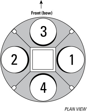
An ADCP measures the Doppler shift of acoustic signals that are reflected by suspended matter within the water column. The water and suspended matter are assumed to be moving at the same velocity. The ADCP used in this study has four acoustic transducers aligned so that the face of each transducer is aimed 20 degrees from perpendicular to the river bottom. The transducers are numbered as shown in figure 2, which shows the transducer as seen from below. If transducer 3 is angled 20 degrees from perpendicular to bottom, oriented toward the bow of the boat, transducer number 4 is angled 20 degrees from perpendicular to bottom, oriented toward the stern of the boat. Likewise, transducers 1 and 2 are angled 20 degrees from perpendicular to bottom, oriented toward port and starboard (left and right side of the boat, as viewed from above, respectively).
Figure 2. Acoustic Doppler current meter (ADCP) transducer configuration (modified from RD Instruments, 1996).
The velocities associated with the acoustic signals emitted by the four transducers are transformed into orthogonal velocity components (ship coordinates) by way of an instrument transformation matrix. This transformation results in velocity vectors in alignment with the current ship heading. If transducer 3 is oriented toward the bow (front) of the boat, the y-axis is then defined as parallel to the keel of the boat, and the x-axis is defined as parallel to the beam of the boat. The z-axis is defined as perpendicular to the bottom of the boat.
In addition to velocities in the x, y, and z directions, an error velocity is reported. The error velocity is scaled so that the variance of the error velocity represents the portion of the variance of each of the x and y components attributable to instrument noise (RD Instruments, 1998).
Most newer ADCP units can be operated in a “pulse-to-pulse coherent” mode. This is a signal-processing technique in which two short pulses are emitted, separated in time by a precisely known lag. The phase difference between the two returned signals is measured. This phase difference is directly proportional to the water velocity (Kim and others, 2000).
The ADCP used in this study uses pulse-to-pulse coherent mode operation, along with improved signal processing, which allows for depth cell sizes as small as 1 cm and increased precision in velocity estimates. In 1 m of water, use of a depth-cell size of 1 cm reportedly results in a single-ping standard deviation in water-velocity measurement of less than 5 cm/s (RD Instruments, 2003).
Although the ADCP unit sends a 1,200-kHz acoustic signal to the stream bottom, the velocity-profile data are recorded less than once per second. Each ping of the sonar generates an instantaneous velocity profile, known as an “ensemble”. To generate an average velocity profile, more than 300 ensembles, or instantaneous velocity profiles, are averaged.
The ADCP cannot accurately measure velocities that are closer than about 6 percent of the total distance between the river bottom and the water surface (RD Instruments, 1996). In other words, in a location where the water depth is 1 m, the closest accurate measurements would be at least 6 cm from the river bottom. This is because echoes from the river bottom are substantially stronger than the echoes from particles in the water column, causing what is known as side-lobe contamination (RD Instruments, 1996). The effect of such contamination of the data is to bias velocities measured within this 6 percent of total depth range toward zero. Because of this effect, the analysis of the data that follows does not consider data collected within this 6 percent of total depth range.
Bottom shear stress is commonly estimated in various ways from velocity data collected near the sediment-water interface. Acoustic Doppler current meters, acoustic Doppler velocimeters, and electromagnetic current meters all have been used to collect the velocity data needed to employ any of the various shear-stress estimation methods.
Shear-stress estimation methods fall into three general categories, based on their treatment of velocity data: first-moment statistics (mean), second-moment statistics (variance), and spectral analysis methods (Kim and others, 2000). In this work, bottom shear stress was estimated by means of both a first-moment and a second-moment method. Shear stress was calculated by several independent methods as a check of one method against the other.
The logarithmic-profile (log-profile) method is a first-moment method, in which the mean flow velocity is related to the distance above the river bottom. The log-profile method applies only to that part of the boundary layer that can be well described by logarithmic functions. The boundary layer has been defined as that part of the water column in which the velocity profile is strongly influenced by the presence of the river bottom, where the flow velocity drops to zero (Carling, 1992). Biron and others (1998) suggest that the boundary layer does not reliably extend above the bottom 20 percent of the flow depth.
The log-profile method was used on two subsets of data from within the boundary layer. The subsets are related to the interval of distance from the sediment bed, and are defined as (1) the subset of points between 6 and 10 percent (6–10 percent subset) of the total flow depth above river bottom and (2) the subset of points between 10 and 20 percent (10–20 percent subset) of the total flow depth above river bottom.
The subset of data that seems most appropriate for application of the log-profile method is the 10–20 percent subset. The reported roughness coefficients and log-profile shear stress are therefore based on the estimates made from the 10–20 percent subset. The profiles within the 6–10 percent interval commonly show influences of bedform and are affected by data contamination near 6 percent of total depth from the river bottom. Nevertheless, velocity-profile plots in the appendix include the log-profile regression results from the 6–10 percent subset so that the reader may compare the results directly.
Within the boundary layer, the mean flow velocity is related to the distance above the river bottom as:
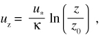 |
(1) |
where uz is the mean flow velocity at a height z above the river bed, u* is the shear velocity, κ is the von Karman constant (≈ 0.41), and z0 is the hydraulic roughness length (Julien, 1998; Carling, 1992).
A subset of data that represents the log layer can be extracted from each velocity profile. A linear regression on this subset of data yields a slope and an intercept value. The slope and intercept values can be used with equation 1 to yield the bottom shear velocity (u*) and hydraulic roughness length (z0):
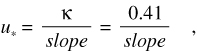 |
(2) |
and
(3) |
Bottom shear stress can then be calculated as
| (4) |
If shear velocity is expressed in centimeters per second and the water density ρ ≈ 1 g/cm3, then the shear stress t is expressed in dynes per centimeter squared (1 dyn/cm2 = 0.1 Pas = 47.88-1 lb/ft2).
The hydraulic roughness, z0, is a mathematical construct with little physical meaning. It represents the height above the sediment bed at which the velocity profile goes to zero. A more physically relevant measure of the sediment bed roughness is called the bottom roughness length (Ks), also known as the grain roughness or the Nikuradse roughness. In an idealized fully rough turbulent boundary layer, the bottom roughness length (Ks) can be estimated as
| (5) |
(Carling, 1992; Cheng and others, 1999).
The value of Ks as defined above should be taken as the minimum value of the bottom roughness. The total bottom roughness may actually include roughness related to benthic organisms (by building mounds or digging burrows), as well as roughness related to the bedform (Courtney K. Harris, Virginia Institute of Marine Science, written commun., 2003).
The turbulent-kinetic-energy (TKE) method relates the absolute intensity of velocity fluctuations to turbulent kinetic energy, which has been related empirically to shear stress (Kim and others, 2000). This method is sensitive to instrument noise and flow-related errors in measurement (Williams and Simpson, 2004).
Turbulent kinetic energy is calculated as
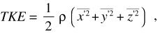 |
(6) |
where ![]() ,
,
![]() ,
and
,
and ![]() are
the average of the calculated velocity variances for a given depth above bottom
and ρ is the density of water (approximately 1 g/cm3) (Stapleton
and Huntley, 1995).
are
the average of the calculated velocity variances for a given depth above bottom
and ρ is the density of water (approximately 1 g/cm3) (Stapleton
and Huntley, 1995).
From the estimate of the turbulent kinetic energy, turbulent shear stress can be estimated as
| (7) |
where C1 is a constant with a value of about 0.19 (Biron and others, 2004; Kim and others, 2000; Stapleton and Huntley, 1995). The specific value of 0.19 used in this work might not apply at all levels within the water column. Kim and others (2000) note that the proportionality constant C1 may need to be confirmed before applying the method universally. Nevertheless, comparing the shear-stress estimates generated by the log-profile and TKE methods yields insight into bottom conditions. Numerous velocity profiles show evidence of possible bedform influence based on the shear stresses estimated from the TKE profile, a finding that would not have been arrived at through the use of the log-profile method alone.
Locations for velocity-profile sampling were selected on the basis of their location relative to proposed sediment-capping locations, and their importance to hydrodynamic model development. This section describes how velocity profiles were captured for each of these sampling locations.
In this work, the ADCP operating mode known as Mode 11 was used for velocity-profile data collection. Mode 11 is recommended for use in shallow water (4 m or less) and low flow velocity (1 m/s or less). Mode 11 yields measurement of velocities with lower standard deviation relative to the other available modes. Mode 11 also allows for smaller water-cell sizes to be measured. In this work, water-cell sizes of 1 cm were used. Other important ADCP configuration settings used in this work are listed in table 2.
Table 2. Project acoustic Doppler current meter (ADCP) configuration.
command |
|
| BM5 | Bottom tracking, set to Mode 5. Recommended for shallow-water environments. |
| WF25 | Blanking distance, set to 25 centimeters. Allows the ADCP transmit circuits to recover before starting the receive cycle. |
| WM11 | Water mode, set to Mode 11. Determines the types of pings that are transmitted. |
| WK1 | Water-cell size, set to 1 centimeter. |
| WN255 | Maximum number of water cells, set to 255. |
| BP2 | Number of bottom pings per ensemble, set to 2. |
| WP1 | Number of water pings per ensemble, set to 1. |
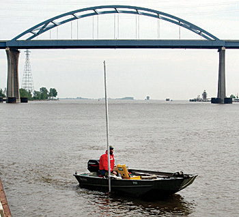
Sampling was done from a 4-meter Jon boat. Sampling locations were recovered by navigating to waypoints stored in a global positioning system (GPS) unit. Upon arrival at each sampling location, the Jon boat was steered into the wind or river current (whichever was stronger at the time). A single anchor at the bow (front) and two anchors off the stern (back) of the boat were used to hold the boat in position.
The ADCP unit was attached to the boat by an adjustable 4-meter aluminum rod. At each sampling location, the length of this rod was adjusted so that the ADCP signal would reach all the way to the river bottom. This distance was recorded as the ADCP offset.
The distance to the center of the first water cell measured by the ADCP is the sum of
To generate water-velocity profile data, an attempt was made to collect at least 300 valid pings or ensembles of data. Collection of the 300 ensembles takes about 5 minutes. Gonzalez-Castro and others (2000) suggest averaging periods of between 5 and 30 minutes to properly characterize mean velocity and turbulence parameters. In the Fox River, a 5-minute averaging period represents an approximate upper practical limit on the averaging period, because of constantly changing flows due to the seiche effect in OU–4.
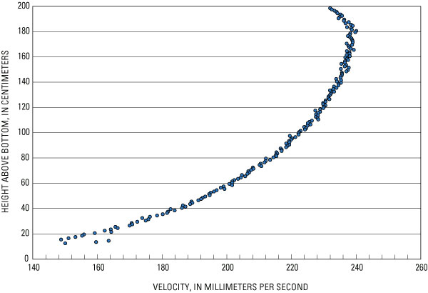
The average velocity profile is generated by averaging all valid velocities for each depth from each ensemble. An example of such a profile is given in figure 3. This figure also demonstrates how forces other than water flow may influence the resulting velocity profile. The curl at the top of the velocity profile in figure 3 is likely caused by the force of the wind acting against the direction of water flow.
Figure 3. Typical velocity profile obtained using the acoustic Doppler current meter (ADCP).
At each sample location, basic information was recorded on a field data sheet, including the name of the electronic data file, the date, time, GPS coordinates of the location, water depth, and ADCP offset.
Water-surface elevations were recorded by means of pressure transducers. For the work in OU–4, five pressure transducers were installed over the length of the reach. For work in OU–3, the number of transducers was reduced to two: one at the upstream end of OU–3 and one at the downstream end.
The pressure transducers were configured to record instantaneous water-level readings every 5 minutes. Separate atmospheric-pressure transducers (that is, non-submerged) were deployed simultaneously to allow corrections for atmospheric-pressure changes. Because of gaps in the resulting atmospheric-pressure transducer data, hourly pressure measurements from the nearby Austin Straubel International Airport were acquired from the NOAA National Climatic Data Center (http://www.ncdc.noaa.gov/oa/climate/climatedata.html#hourly).
Traditional level-loop and GPS survey instruments were used to establish reference point (RP) elevations relative to the NGVD 88. All benchmarks used in this report were generated on behalf of the Wisconsin Department of Natural Resources for use on Fox River-related projects. These benchmark elevations were uniformly established relative to NGVD 88 (RETEC Group, Inc., 2004).
Measurements between the reference point elevation and the water surface were made approximately monthly. These measurements were used to transform the arbitrary levels recorded by the pressure transducer into water-surface elevations relative to the known reference point elevations.
Velocity-profile data were processed by use of custom software (ADCPREAD) developed for this project. The software is written in the Perl language. Customized software was developed because the standard software provided with the ADCP is designed primarily for discharge measurements and does not provide a straightforward way to generate shear velocity and stress estimates.
The ADCPREAD software performs the following data-processing steps:
A velocity result was judged to be invalid if any of the beams reported indeterminate values (-32768) or if the ADCP was forced to make a calculation using only three beams. An ensemble was judged invalid if any of the associated bottom-tracking data were flagged as bad.
Velocity profiles were identified as invalid if any of the following criteria were true:
A separate Perl program was used to generate and execute a command file using the R statistical software package. R is an open-source version of the S statistical language and includes a wide variety of statistical and graphical analysis tools (R Development Core Team, 2006). The R package was used to generate shear-stress estimates using both the log-profile method and the TKE method.
The log-profile method was implemented by plotting a subset of the measured average velocity against the natural log of the depth above bottom. Shear-stress parameters were calculated for the 6–10 percent and 10–20 percent depth-above-bottom subsets of all velocity-profile data.
A linear regression on these data subsets yielded a slope and an intercept value for each. From this linear regression, the bottom shear velocity (u*) and hydraulic roughness length (z0) were calculated using equations 2 and 3.
A 95-percent confidence interval about the shear-velocity estimate was estimated within the R statistics package using the method described in Cheng and others (1999):
| (8) |
with ![]() given
as
given
as
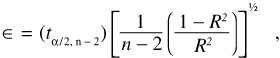 |
(9) |
In the equation above, t is the quantile of the Student’s t-distribution for the 1–a confidence interval for a given number of degrees of freedom, n is the number of velocity data points included in the linear regression, and R2 is the regression correlation coefficient.
The TKE method begins with the TKE as calculated by use of equation 6. Because the method is sensitive to instrument noise, estimated instrument noise was subtracted from the turbulence statistics.
Two procedures have been suggested for removing instrument noise from the TKE calculation if ADCPs are the source of velocity data (Williams and Simpson, 2004; Stacey and others, 1999). Unfortunately, both of these procedures are geared to situations in which velocity data are recorded in beam coordinates; in other words, to data sets where velocities are recorded relative to the orientation of each of the four beams of the ADCP. In this work, all velocities were recorded relative to ship coordinates, which made these procedures impracticable. Therefore, alternative procedures were used to estimate and remove instrument noise from the calculated variances.
At some point above the river bottom within the water column, turbulent kinetic energy is assumed to be zero. Using this assumption, an error (or noise) term for the velocity components is calculated as given by equation 10. Formulations for the y and z components are identical in form.
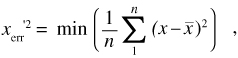 |
(10) |
In equation 10, xerr'2 is the minimum variance
in calculated water velocities for all depth cells, ![]() is
the average water velocity calculated from all valid ensembles for a given water
cell, x is the water velocity for a specific ensemble,
and n is the number of valid ensembles included in the calculation.
is
the average water velocity calculated from all valid ensembles for a given water
cell, x is the water velocity for a specific ensemble,
and n is the number of valid ensembles included in the calculation.
Subsequently, the error term presented above (assumed to represent variance due to instrument noise) was subtracted from the variance as calculated for the vertical velocity components, as shown in equation 11. The formulations for the other two velocity components can be described by substituting y or z for x in equation 11.
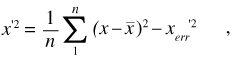 |
(11) |
The shear stresses reported under the heading “calculated shear-stress parameters” on the plots included in the appendix were calculated as described below.
The average of the variance terms was calculated for the subset of water cells between 6 and 10 percent of the total flow depth above the bottom. These terms were used to calculate turbulent kinetic energy using equation 6. The bottom shear stress was estimated from the turbulent kinetic energy using equation 7. The specific calculation interval, 6 to 10 percent of total depth, was chosen to smooth out spikes of TKE from the depth band closest to the sediment-water interface.
One of the main goals of this project was to provide field-data support for possible development of a numerical hydrodynamic model. Such a model could be used to characterize shear stress above the sediment deposits that are the most likely candidates for sediment capping. The coefficient of friction, Cf, is used in the numerical model to estimate shear stress from predicted velocities. Cf can be defined as
 |
(12) |
where ![]() s
the vertically averaged water velocity at the point of ADCP deployment (cm/s), t is
the bottom shear stress (dyn/cm2),
and ρ is the water density
(about
1 g/cm3).
s
the vertically averaged water velocity at the point of ADCP deployment (cm/s), t is
the bottom shear stress (dyn/cm2),
and ρ is the water density
(about
1 g/cm3).
The water-level loggers used in the study were unvented, which means that changes in local atmospheric pressure would bias the water-level readings. The first step in processing the water-level data was to correct for the effects of local atmospheric pressure. The second step in this process was to tie the water-level data to a common datum.
Atmospheric pressure data from Austin Straubel Field in Green Bay were used for corrections to the water-level data. To account for the elevation difference between the airport monitoring site and the water-level stations, the following equation was used:
 |
(13) |
where h is the elevation difference between two pressure recording stations (meters), T is the average air temperature of the layer of the atmosphere (degrees Kelvin), K is the universal gas constant (287 J/kg/°K), g is the acceleration due to gravity (9.8 m/s2), p0 is the pressure of the station at the lower altitude, and p1 is the pressure of the station at the higher altitude. The equation was solved for p0 or p1, depending on whether the transducer site was higher or lower than the airport.
The barometric-pressure effects on water level are as follows: 1 mbar = 10.2 mm of water = 0.0102 m of water. For example, given a barometric pressure change of 900 mbar to 910 mbar, the equivalent change in water level is 10 mbar times 0.0102 m, or 0.1 m.
The uncorrected transducer stage record was corrected for atmospheric-pressure fluctuations by comparing the atmospheric pressure at the time of each reading to the atmospheric pressure at the time the level logger was started. The change in atmospheric pressure for each reading was converted to an equivalent water depth and added to or subtracted from the uncorrected stage to obtain a corrected stage.
Once the local reference-point elevation was established relative to NAVD 88, it was converted to IGLD 85 by following a two-step process (Coordinating Committee, 1995; Jeff Oyler, National Oceanic and Atmospheric Administration, written commun., 2005):
Water-elevation data in OU–4 relative to NGVD 88 were converted to an elevation relative to IGLD 85 by converting the orthometric height to a dynamic height and subtracting the hydraulic corrector.
This section presents the results of the 109 valid velocity profiles obtained on the Lower Fox River, as well as the recorded water levels. Results are discussed separately for OU–3 and OU–4.
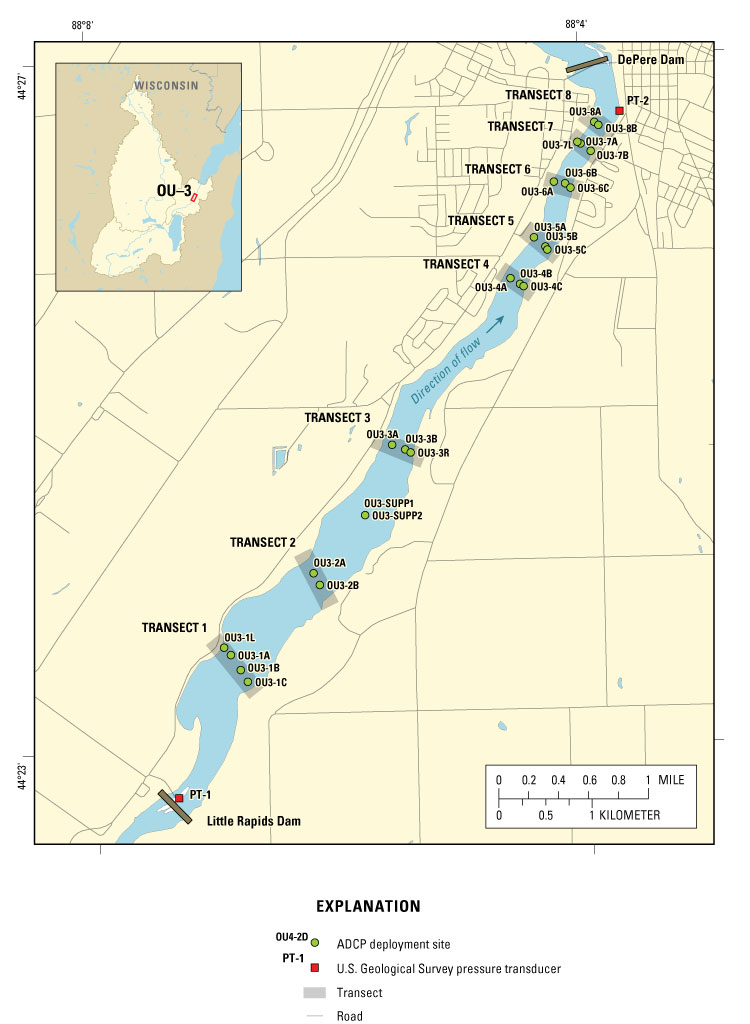
ADCP deployment sites with valid profiles for OU–3 are shown in figure 4.
Figure 4. Acoustic Doppler current meter (ADCP) deployment sites with valid profiles within Operable Unit 3, Lower Fox River, Wis.
Water levels in OU–3 during September and October varied by several feet. Water levels rose by nearly a foot on about October 26, when the Corps of Engineers opened dam gates at Neenah and Menasha.
The rapid fluctuations in water levels within OU–3 are largely the result of hydroelectric-power operations on the river, which include the Kaukauna Electric facilities upstream and the Nicolet Paper Company at the DePere Dam downstream. The OU–3 reach of the Lower Fox River appears to function as a level-pool reservoir; there is minimal change in the slope of the water-surface elevation between the upstream and downstream pressure transducers (figure 5).
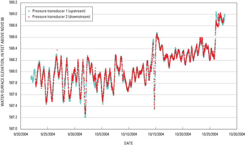
Figure 5. Recorded water-surface elevations in Operable Unit 3, September and October 2004.
Velocity profiles for a single event were obtained for OU–3 on October 26 and 27, 2004. The daily average discharge at the Appleton streamflow-gaging station (04084445) was about 7,700 ft3/s (218 m3/s). By comparison, the discharge associated with a 2-year recurrence interval is 12,600 ft3/s (357 m3/s).
Of the 33 profiles for which data were collected, 31 (94 percent) were categorized as valid. Table 3 summarizes the hydraulic and turbulence parameters calculated for the vertical velocity profiles. Individual profiles are found in the appendix.
Table 3. Summary statistics, Operable Unit 3 velocity profiles, October 2004.
[ft, foot; ft/s, foot per second; cm, centimeter; cm/s, centimeter per second; LP, log profile; %, percent; TKE, turbulent kinetic energy; Ks, bottom roughness length; Cf, coefficient of friction; shear stress values in dynes per square centimeter]
| Average depth (ft) | ||||||
| Averge velocity (ft/s) | ||||||
| Shear velocity (cm/s) | ||||||
| Shear stress (LP, 10–20%) | ||||||
| Shear stress (LP, 6–10%) | ||||||
| Shear stress (TKE) | ||||||
| Ks (cm) | ||||||
| Cf |
The average shear stress calculated using the TKE method was higher than that calculated with the log-profile method. This is true only for the October 2004 velocity profiles. In all other cases, the TKE method produced a shear-stress estimate that was less than that estimated by the log-profile method. Biron and others (2004) found that in their work, the log-profile method generally produced the largest estimated shear stress value, with the TKE method producing average estimates about 30 percent less than the log-profile-method estimates.
ADCP deployment sites with valid profiles for OU–4 are shown in figure 6.
Figure 6. Acoustic Doppler current meter (ADCP) deployment sites with valid profiles within Operable Unit 4, Lower Fox River, Wis.
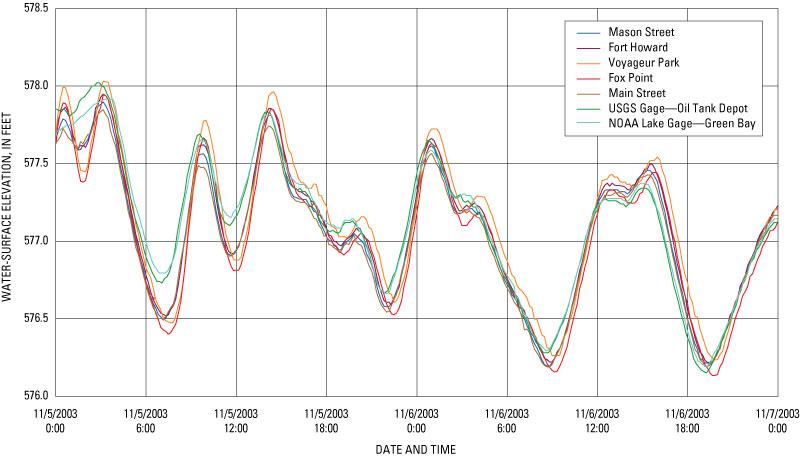
Figure 7 shows a typical water-surface elevation data set from OU–4. In general, the sites located furthest upstream exhibit the widest swings between minimum and maximum water-surface elevations. Not surprisingly, peak values at the sites that are furthest upstream are lagged in time relative to water-surface-elevation changes in Green Bay.
Figure 7. Example of measured water-surface-elevation fluctuations at all measurement sites, Lower Fox River, Wis., November 5–7, 2003.
Changes in water-surface elevations in Green Bay (NOAA and USGS gages) appear to take as much as an hour to be reflected in the observations at the water-elevation sites furthest upstream (Voyageur Park and Fox Point gages). Differences of about 0.1 ft might not be significant, however, due to the level of accuracy of the GPS survey used to determine the elevations of the reference points.
Approximately 107 velocity profiles were generated in the four ADCP deployments for OU–4. As can be seen in table 4, deployments in areas with water depths ranging from about 4 ft to 12 ft produced the greatest number of valid profiles.
Table 4. Summary of velocity profiles by water depth.
[≥, greater than or equal to; <, less than]
Number |
Valid profiles |
|||
Deployments in shallow water (less than 4 ft) and in deep water (greater than 18 ft) yielded the lowest proportion of valid profiles relative to deployments in areas of intermediate water depth (between 4 and 18 feet of water).
Velocity profiles were obtained between June 24 and June 27, 2003. The daily average discharge at the Appleton streamflow-gaging station (04084445) was about 3,800 ft3/s (108 m3/s).
Of the 24 profiles for which data were collected, 12 (50 percent) were categorized as valid. Table 5 summarizes the hydraulic and turbulence parameters calculated for the vertical-velocity profiles. Individual profiles are in the appendix.
Table 5. Summary statistics, Operable Unit 4 velocity profiles, June 2003, Lower Fox River, Wis.
[ft, foot; ft/s, foot per second; cm, centimeter; cm/s, centimeter per second; LP, log profile; %, percent; TKE, turbulent kinetic energy; Ks, bottom roughness length; Cf, coefficient of friction; shear stress values in dynes per square centimeter]
deviation |
||||||
| Average depth (ft) | ||||||
| Average velocity (ft/s) | ||||||
| Shear velocity (cm/s) | ||||||
| Shear stress (LP, 10–20%) | ||||||
| Shear stress (LP, 6–10%) | ||||||
| Shear stress (TKE) | ||||||
| Ks (cm) | ||||||
| Cf |
The June 2003 sampling event was designed as a “shakedown cruise” to test the configuration of hardware and software used to collect the velocity-profile data. Only one of the valid profiles was collected using Mode 11. All other velocity profiles were collected using Mode 5, with 5-cm water cells. Mode 5 generally produces noisier data than Mode 11 does, and along with the relatively large water-cell sizes, noise could be part of the reason for the low number of valid profiles generated from this sampling.
Velocity profiles were obtained on November 5 and 6, 2003. The daily average discharge at the Appleton streamflow-gaging station (04084445) was about 7,100 ft3/s (201 m3/s).
Of the 32 profiles for which data was collected, 20 (63 percent) were categorized as valid. Table 6 summarizes the hydraulic and turbulence parameters calculated for the vertical-velocity profiles. Individual profiles are included in the appendix.
Table 6. Summary statistics, Operable Unit 4 velocity profiles, November 2003, Lower Fox River, Wis.
[ft, foot; ft/s, foot per second; cm, centimeter; cm/s, centimeter per second; LP, log profile; %, percent; TKE, turbulent kinetic energy; Ks, bottom roughness length; Cf, coefficient of friction; shear stress values in dynes per square centimeter]
deviation |
||||||
| Average depth (ft) | ||||||
| Average velocity (ft/sec) | ||||||
| Shear velocity (cm/sec) | ||||||
| Shear stress (LP, 10–20%) | ||||||
| Shear stress (LP, 6–10%) | ||||||
| Shear stress (TKE) | ||||||
| Ks(cm) | ||||||
| Cf |
Velocity profiles were obtained March 6 and March 8, 2004. The daily average discharge at the Appleton streamflow-gaging station (04084445) was about 10,800 ft3/s (305 m3/s).
Of the 26 profiles for which data were collected, 15 (58 percent) were categorized as valid. Table 7 summarizes the hydraulic and turbulence parameters calculated for the vertical-velocity profiles. Individual profiles are included in the appendix.
Table 7. Summary statistics, Operable Unit 4 velocity profiles, March 2004, Lower Fox River, Wis.
[ft, foot; ft/s, foot per second; cm, centimeter; cm/s, centimeter per second; LP, log profile; %, percent; TKE, turbulent kinetic energy; Ks, bottom roughness length; Cf, coefficient of friction; shear stress values in dynes per square centimeter]
| Count | deviation |
|||||
| Average depth (ft) | ||||||
| Average velocity (ft/sec) | ||||||
| Shear velocity (cm/sec) | ||||||
| Shear stress (LP, 10–20%) | ||||||
| Shear stress (LP, 6–10%) | ||||||
| Shear stress (TKE) | ||||||
| Ks(cm) | ||||||
| Cf |
Velocity profiles were obtained between May 25 and May 27, 2004. The daily average discharge at the Appleton streamflow-gaging station (04084445) was about 14,600 ft3/s (413 m3/s). This discharge is slightly less than the discharge associated with the 5-year recurrence interval (15,100 ft3/s (428 m3/s).
Of the 35 profiles for which data were collected, 27 (77 percent) were categorized as valid. Table 8 summarizes the hydraulic and turbulence parameters calculated for the vertical-velocity profiles. Individual profiles are included in the appendix.
Table 8. Summary statistics, Operable Unit 4 velocity profiles, May 2004, Lower Fox River, Wis.
[ft, foot; ft/s, foot per second; cm, centimeter; cm/s, centimeter per second; LP, log profile; %, percent; TKE, turbulent kinetic energy; Ks, bottom roughness length; Cf, coefficient of friction; shear stress values in dynes per square centimeter]
| Count | deviation |
|||||
| Average depth (ft) | ||||||
| Average velocity (ft/sec) | ||||||
| Shear velocity (cm/sec) | ||||||
| Shear stress (LP, 10–20%) | ||||||
| Shear stress (LP, 6–10%) | ||||||
| Shear stress (TKE) | ||||||
| Ks(cm) | ||||||
| Cf |
In OU–3, several of the shear-stress estimates made with the TKE method exceeded those made with the log-profile method. The initial thought was that perhaps the sampling had captured turbulent energy related to the wave activity within OU–3. On October 26, winds averaged from 12 to 16 mi/h (19−26 km/h), from the northeast (180º opposite the flow direction). Langmuir current spirals and 1- to 1.5-ft waves were observed during the data collection.
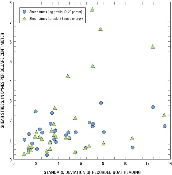
Closer inspection of the ADCP logs reveals that the profiles for which the TKE method produced shear-stress estimates higher than the log-profile-method estimates were also the profiles for which the boat crew had the most difficulty maintaining a constant heading. It seems more likely that the bulk of the excess shear stress estimated using the TKE method is due to apparent turbulence induced by excessive boat movement and not due to orbital wave velocities. Figure 8 shows that the two methods track reasonably well until the standard deviation in the boat heading approaches 4. For standard deviations in heading greater than 4, the TKE method appears to yield a shear-stress estimate somewhat greater than that estimated from the log-profile method.
Figure 8. Log-profile (LP) and total-kinetic-energy (TKE) estimates of shear stress for various standard deviations in heading, Operable Unit 3, Lower Fox River, Wis.
The standard deviation in heading is a surrogate for general boat motions. A relation similar to that shown in figure 8 was found between the calculated TKE shear stress and the standard deviation in pitch and roll of the ADCP unit as well.
Although the crew attempted to minimize all boat and ADCP movement during velocity-profile data collection, such movement was unavoidable during periods of gusty wind. It appears that second-order shear-stress estimation methods, such as the TKE method, may be sensitive to excessive boat movements.
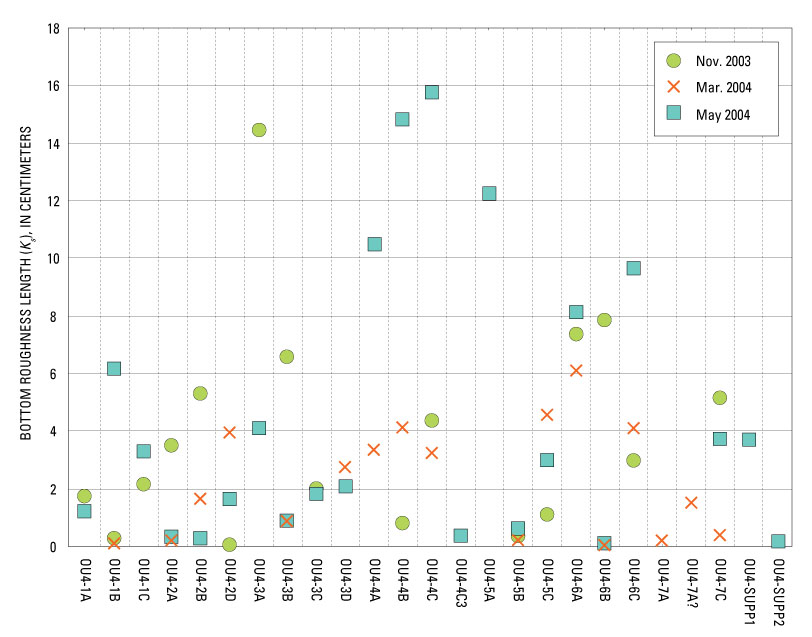
Roughness lengths (Ks) were calculated for all valid profiles on the basis of the log-profile method, using velocity points falling within a distance of between 10 and 20 percent of the total water depth from the sediment bed. Table 9 summarizes the calculated Ks values.
Table 9 and figure 9 show fairly consistent average values of Ks for OU–4 during the November 2003 and the March and May 2004 samplings. By contrast, the June 2003 ADCP deployment in OU–4 resulted in Ks estimates about 9 times greater.
Table 9. Roughness lengths for all acoustic Doppler current meter (ADCP) deployment events, Lower Fox River, Wis.
[ft/s, feet per second; cm, centimeter]
June 2003 |
||||||
November 03 |
||||||
March 2004 |
||||||
May 2004 |
||||||
October 2004 |
||||||
Figure 9. Estimated roughness lengths, OU–4, Lower Fox River, Wis.
In June 2003, most of the velocity profiles were collected using ADCP Mode 5 and a 5-cm water-cell size. The bulk of the remainder of the profiles in both OU–3 and OU–4 were obtained using ADCP Mode 11 and a 1-cm water-cell size. It appears that the specific shear-stress parameter estimates resulting from the methods described in this report are highly related to the choice of ADCP data-collection mode and water-cell size.
Estimated Ks values for OU–3 appear to be greater than those estimated for OU–4. The average and median values for OU–3 are between 2 and 3 times those estimated for OU–4. There is no clear explanation regarding why there should be differences in Ks between OU–3 and OU–4.
OU–3 is not subject to the seiche activity, storm surges, and long-term lake-level fluctuations that affect OU–4. OU–3 is also a much wider and somewhat shallower basin than OU–4. These facts may be related to the differing estimates of Ks between the two operable units.
This section presents a series of tables (tables 10–13) summarizing the main shear-stress parameters that were estimated from the velocity-profile data. The October 2004 dataset pertains specifically to OU–3; all other deployment dates pertain to OU–4.
Table 10. Vertically averaged velocity for all events, Lower Fox River, Wis.
[ft/s, feet per second; ft3/s, cubic feet per second]
discharge (ft3/s) |
||||||
June 2003 |
||||||
November 2003 |
||||||
March 2004 |
||||||
May 2004 |
||||||
October 2004 |
||||||
Table 11. Shear stress by log-profile (LP) method, 10–20 percent of depth, for all events, Lower Fox River, Wis.
[ft/s, feet per second; dyn/cm2, dynes per square centimeter]
discharge (ft3/s) |
||||||
June 2003 |
||||||
November 2003 |
||||||
March 2004 |
||||||
May 2004 |
||||||
October 2004 |
||||||
Table 12. Shear stress by turbulent-kinetic-energy (TKE) method for all events, Lower Fox River, Wis.
[ft/s, feet per second; dyn/cm2, dynes per square centimeter]
discharge (ft3/s) |
||||||
June 2003 |
||||||
November 2003 |
||||||
March 2004 |
||||||
May 2004 |
||||||
October 2004 |
||||||
Table 13. Shear stress by log-profile (LP) method, 6–10 percent of depth, for all events, Lower Fox River, Wis.
[ft/s, feet per second; dyn/cm2, dynes per square centimeter]
discharge (ft3/s) |
||||||
June 2003 |
||||||
November 2003 |
||||||
March 2004 |
||||||
May 2004 |
||||||
October 2004 |
||||||
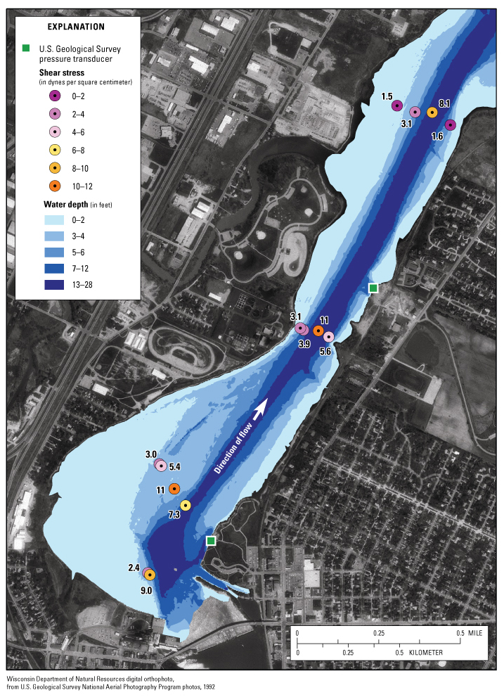
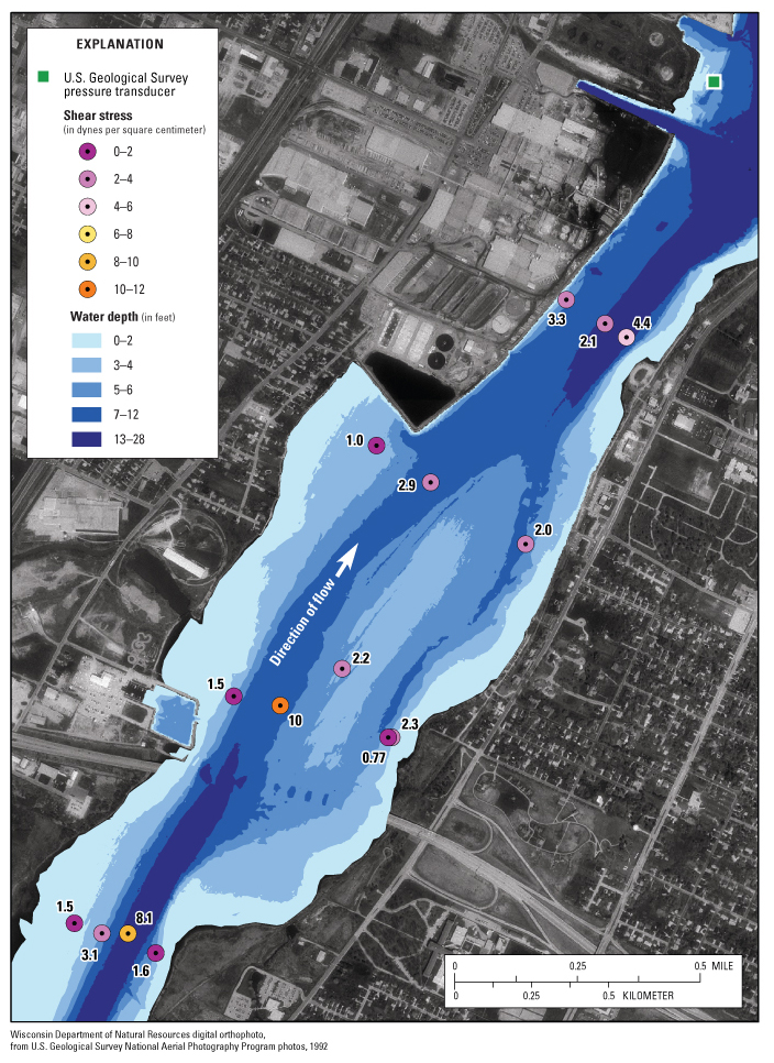
The spatial distribution of estimated shear-stress values in a part of OU−4 is shown in figures 10a and 10b for the May 2004 ADCP deployment. In general, the highest estimates of shear stress were found where one would expect them: in the areas of highest river velocity. In most cases, these areas correspond to the deepest parts of the river, as can be seen in figures 10a and 10b.
Figure 10a. Distribution of calculated shear stress during May 2005 sampling event, Operable Unit 4 (transects 1 through 3), Lower Fox River, Wis. Bathymetry is from the work completed by Jenkins Survey and Design under contract to Wisconsin DNR (October, 2004).
Figure 10b. Distribution of calculated shear stress during May 2005 sampling event, Operable Unit 4 (transects 3 through 6), Lower Fox River, Wis. Bathymetry is from the work completed by Jenkins Survey and Design under contract to Wisconsin DNR (October, 2004).
Some of the highest shear-stress estimates are in OU−4 at transect 2, at the narrowest part of the river downstream from De Pere. Other areas with high estimated shear stresses are found in or adjacent to the turning basin and navigation channel, which appear in figures 10a and 10b in darker shades of blue. Water depths are given relative to the low water datum of 577.5 ft (IGLD 85) for Lake Michigan.
One of the objectives of the study described here was to provide data that could be used in support of a hydrodynamic modeling effort. In a hydrodynamic model application, a coefficient of friction is typically defined in order to calculate the bottom shear stress. The bottom shear stress in a river balances the downstream momentum of flow. Thus, the value of the coefficient of friction directly influences model-predicted velocity fields and shear stresses. The coefficient of friction is directly proportional to the bottom shear stress divided by the square of the vertically averaged flow velocity.
The law-of-the-wall relation (eq. 1) can be rewritten to produce an estimate of the bottom friction coefficient:
 |
(14) |
where z is the total water depth, z0 is the hydraulic roughness length, and κ is the von Karman constant (≈ 0.41). From equation 14, one can see that the coefficient of friction increases as the roughness length increases or as the water depth decreases.
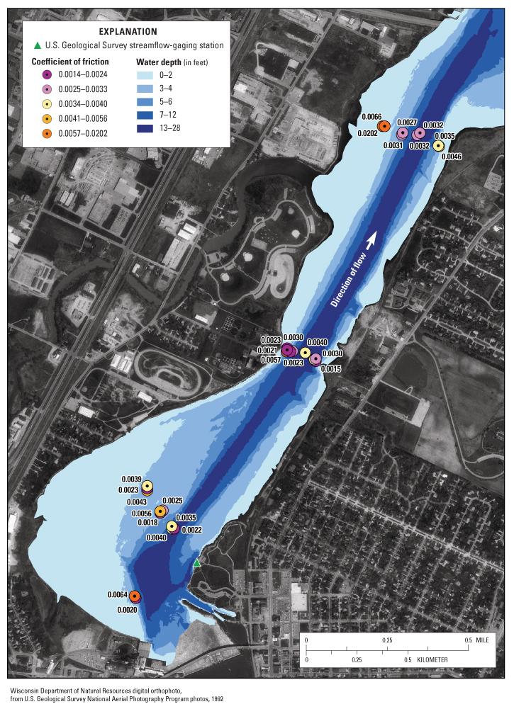
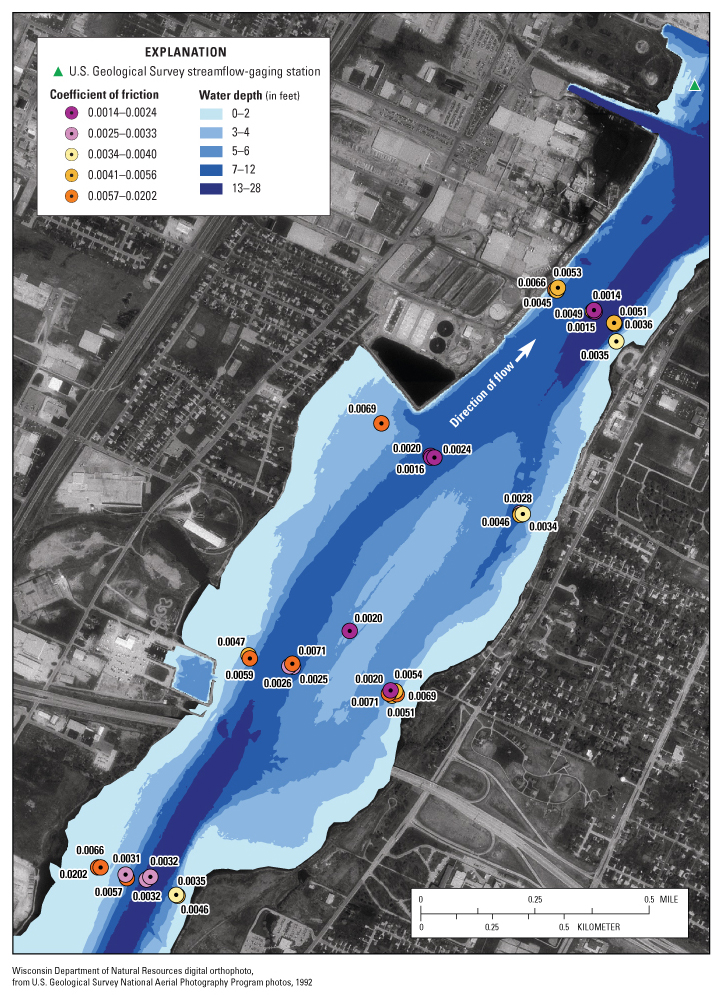
The spatial distribution of the bottom coefficient of friction for OU–4 is shown in figures 11a and 11b.
Figure 11a. Distribution of the bottom coefficient of friction calculated from November 2003 and March and May 2004 profiles, Operable Unit 4 (transects 1 through 3), Lower Fox River, Wis. Bathymetry is from the work completed by Jenkins Survey and Design under contract to Wisconsin DNR (October, 2004).
Figure 11b. Distribution of the bottom coefficient of friction calculated from November 2003 and March and May 2004 profiles, Operable Unit 4 (transects 3 through 6), Lower Fox River, Wis. Bathymetry is from the work completed by Jenkins Survey and Design under contract to Wisconsin DNR (October, 2004).
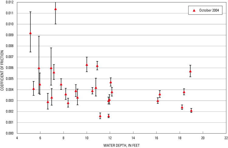
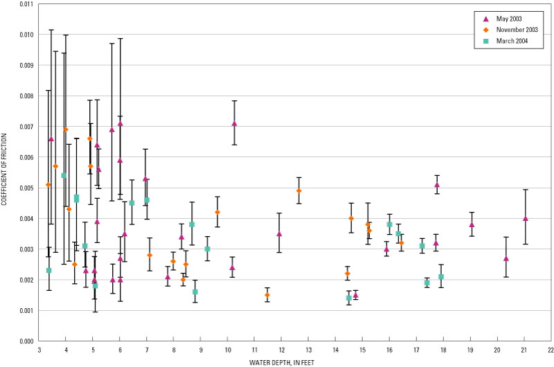
The relation between the calculated coefficients of friction and the water depth at the ADCP deployment sites in OU−3 and OU−4 is shown in figures 12 and 13.
Figure 12. Variation in the bottom coefficient of friction with depth in Operable Unit 3, Lower Fox River, Wis.
Figure 13. Variation in the bottom coefficient of friction with depth in Operable Unit 4, Lower Fox River, Wis.
In figures 12 and 13, the error bars are calculated by using the upper and lower bounds of the 95-percent confidence interval about the estimated shear stress and calculating the upper and lower bounds of the coefficient of friction by means of equation 11.
Clearly, water depth is not the only factor explaining the variation in the calculated coefficient of friction. In addition to spatial variations, some sites show an apparent increase in calculated coefficients of friction over time. Many of these sites also show signs of the presence of bedforms, as evidenced by a peak in the associated TKE-estimated shear-stress profiles. It is possible that the higher flows observed during the May 2004 deployment resulted in more active bed movement, and, hence, increases in the calculated coefficients of friction.
Deployment sites were too few, however, to allow for spatial interpolation of the coefficients of friction.
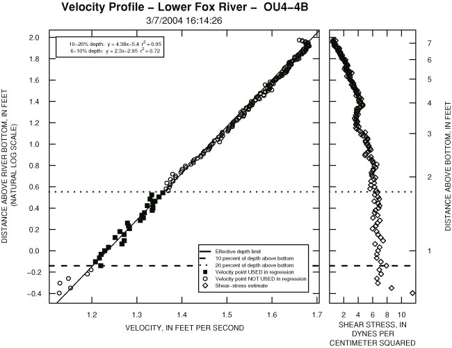
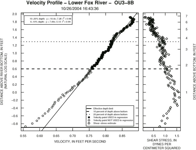
Under ideal conditions, taking the natural log of the distance above the sediment bed and plotting this distance against the average velocity results in a relation that approximates a straight line, as in figure 14.
Figure 14. Example of a close-to-ideal velocity profile.
During the course of this project, two types of velocity profiles that depart significantly from the ideal were identified: (1) those for which significant influence of the wind is apparent in the velocity profile, and (2) those for which two-dimensional bedforms, such as ripples or mounds, appear to influence both the shear-stress and velocity profiles.
Figure 15 shows a profile that is strongly influenced by winds. At the time of ADCP deployment, the wind was roughly 9 mi/h in a direction opposite to river flow. The resulting velocity profile shows the apparent effect of the wind as the profile curls back as the distance to the water surface decreases. The water depth for the site depicted in figure 15 is about 7.2 ft.
Figure 15. Example of a velocity profile strongly influenced by the wind.
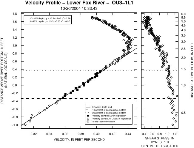
Figure 16 is an example of the second common deviation from the idealized velocity profile, one that reflects the effects of two-dimensional bedforms. These bedforms may include structures such as ripples, mounds, and dunes. Channel modifications, such as dredged navigational channels and turning basins, could also produce similar deviation from the idealized velocity profile.
Figure 16. Example of a velocity profile showing possible bedform influences.
Nelson and others (1993) studied how two-dimensional bedforms affect velocity and shear-stress distributions. They found that both upstream and downstream from a two-dimensional bedform, the shear stress increased “away from the bed in the near-bed wake region, reaching a maximum at the center of the wake region, and decreasing to zero at the water surface” (Nelson and others, 1993). The shear-stress and velocity profiles shown in figure 16 clearly seem to reflect the influence of two-dimensional bedforms (ripples, mounds, or dunes).
It is possible that the break in the boundary layer structure seen in several profiles is due in part to side-lobe contamination of the ADCP measurements in the water layer immediately above the bed. For profiles such as the one shown in figure 16, however, the break appears to be well above the effective depth limit of the ADCP, and likely truly reflects the influence of a bedform structure.
Replicate datasets were collected during each ADCP deployment for a subset of locations. The intent of acquiring replicate datasets was to gain an idea of how precise any given estimate at a point might be.
Estimates of shear stress calculated from replicate data sets are compared in tables 14 and 15; estimates of bottom roughness (Ks) from the replicate data sets are compared in table 16. In each table, a subjective label has been assigned to each replicate based on the type of velocity-depth profile that is present. These types are “ideal,” “bedform,” and “wind,” as defined in the previous section of this report.
Table 14. Comparison of replicate shear-stress estimates by the log-profile method.
[mm/dd/yyyy, month/day/year; dyn/cm2, dyne per square centimeter]
Transect |
(mm/dd/yyyy) |
difference (percent) |
|||
| OU4-1C | Ideal | ||||
| OU4-1A | Bedform | ||||
| OU4-SUPP1 | Bedform | ||||
| OU4-4C | Bedform | ||||
| OU3-1L | Wind | ||||
| OU3-1B | Ideal | ||||
| OU3-2A | Ideal | ||||
| OU3-6B | Ideal | ||||
| OU3-6A | Ideal | ||||
| OU3-5B | Bedform | ||||
| OU3-5A | Wind and bedform | ||||
median: 48 |
|||||
| profiles only): 38 |
|||||
Table 15. Comparison of replicate shear-stress estimates by the turbulent-kinetic-energy (TKE) method.
[mm/dd/yyyy, month/day/year; dyn/cm2, dyne per square centimeter]
(mm/dd/yyyy) |
difference (percent) |
||||
| OU4-1C | Ideal | ||||
| OU4-1A | Bedform | ||||
| OU4-SUPP1 | Bedform | ||||
| OU4-4C | Bedform | ||||
| OU3-1L | Wind | ||||
| OU3-1B | Ideal | ||||
| OU3-2A | Ideal | ||||
| OU3-6B | Ideal | ||||
| OU3-6A | Ideal | ||||
| OU3-5B | Bedform | ||||
| OU3-5A | Wind and bedform | ||||
| median: 19 | |||||
| median (ideal profiles only): 18 |
|||||
Table 16. Comparison of replicate roughness length (Ks) estimates.
[mm/dd/yyyy, month/day/year; cm, centimeter]
(mm/dd/yyyy) |
difference (percent) |
||||
| OU4-1C | Ideal | ||||
| OU4-1A | Bedform | ||||
| OU4-SUPP1 | Bedform | ||||
| OU4-4C | Bedform | ||||
| OU3-1L | Wind | ||||
| OU3-1B | Ideal | ||||
| OU3-2A | Ideal | ||||
| OU3-6B | Ideal | ||||
| OU3-6A | Ideal | ||||
| OU3-5B | Bedform | ||||
| OU3-5A | Wind and bedform | ||||
profiles only): 98 |
|||||
Replicates with the highest relative percent difference in shear-parameter estimates tend to be those for which velocity profiles departed from the ideal log profile.
The estimate of shear stress by the TKE method has the lowest relative percent difference between replicates, with a median difference of 19 percent. Estimates of shear stress made using the log-profile method have a median relative percent difference of 48 percent.
The bottom roughness estimate replicates have the largest relative percent differences. Particularly for the replicates that clearly are influenced by bedforms, the differences in estimated bottom roughness could be due to increased heterogeneity in bottom materials near bedform features.
An acoustic Doppler current profiler (ADCP) mounted on a moored vessel was used to generate velocity profiles in two discrete areas, or “operable units” of the Lower Fox River near Green Bay, Wisconsin. This method of data collection yielded 158 velocity profiles from Operable Units 3 and 4 on the Lower Fox River between June 2003 and November 2004. Of these profiles, 109 were classified as valid and were used to calculate the bottom shear stress and velocity using two estimation methods—log-profile and turbulent-kinetic-energy (TKE). Velocity-profile data were collected over a range of hydraulic conditions, with maximum river flows just below the discharge associated with the 5-year recurrence interval.
In Operable Unit 3, estimated shear stress ranged from 0.09 to 2.87 dyn/cm2. Estimated coefficients of friction ranged from 0.002 to 0.011. Recorded flow velocities ranged from 0.3 to 0.87 ft/s.
In Operable Unit 4, estimated shear stress ranged from 0.09 to 10.8 dyn/cm2. Estimated coefficients of friction ranged from 0.001 to 0.007, excluding calculations made using the June 2003 data. Recorded flow velocities ranged from 0.09 to 1.71 ft/s.
Several conclusions may be drawn from this work:
Biron, P., Robson, C., Lapointe, M., and Gaskin, S., 2004, Comparing different methods of bed shear stress estimates in simple and complex flow fields: Earth Surface Processes and Landforms, v. 29, p. 1403–1415.
Biron, P., Lane, S., Roy, A., Bradbrook, K., and Richards, K., 1998, Sensitivity of bed shear stress estimated from vertical velocity profiles—The problem of sampling resolution: Earth Surface Processes and Landforms, v. 23, p. 133–139.
Carling, P., 1992, The nature of the fluid boundary layer and the selection of parameters for benthic ecology: Freshwater Biology, v. 28, p. 273–284.
Cheng, R., Ling, C., Gartner, J., and Wang, P., 1999, Estimates of bottom roughness length and bottom shear stress in South San Francisco Bay, California: Journal of Geophysical Research, v. 104, no. C4, p. 7715–7728.
Coordinating Committee on Great Lakes Basic Hydraulic and Hydrologic Data (Coordinating Committee), 1995, Establishment of International Great Lakes Datum (1985): Chicago, Ill., and Ottawa, Ont., accessed November 8, 2006 at http://www.lre.usace.army.mil/greatlakes/hh/links/ccglbhhd/committeepublications/
Gargett, A., 1994, Observing turbulence with a modified acoustic Doppler current profiler: Journal of Atmospheric and Oceanic Technology, v. 11, p. 1592–1610.
Gonzalez-Castro J., Oberg K., and Duncker J., 2000, Effect of temporal resolution on the accuracy of ADCP measurements, in Proceedings of the American Society of Civil Engineers 2000 Joint Conference on Water Resource Engineering and Water Resources Planning, July 30–August 2: Minneapolis, Minn., CD-ROM.
Julien, P.Y., 1998, Erosion and sedimentation: Cambridge, England, Cambridge University Press, 280 p.
Kim, S., Friedrichs, C., Maa, J., and Wright, L., 2000, Estimating bottom stress in tidal boundary layer from acoustic Doppler velocimeter data: Journal of Hydraulic Engineering, v. 126, p. 399–406.
Nelson, J.M., McLean, S.R., and Wolfe, S.R., 1993, Mean flow and turbulence fields over two-dimensional bedforms: Water Resources Research, v. 29 no. 12, p. 3935–3954.
R Development Core Team, 2006, R: A language and environment for statistical computing, R Foundation for Statistical Computing: Vienna, Austria, ISBN 3-900051-07-0, accessed November 8, 2006 at http://www.R-project.org/
RD Instruments, 1996, Acoustic Doppler current profiler—principles of operation, a practical primer (2nd ed. for broadband ADCPs): RD Instruments, San Diego, Calif., P/N 951-6069-00, 52 p.
RD Instruments, 1998, ADCP coordinate transformation—formulas and calculations: RD Instruments, San Diego, Calif., P/N 951-6079-00, 29 p.
RD Instruments, 2001, Workhorse commands and output data format: RD Instruments, San Diego, Calif., P/N 957-6156-00, 158 p.
RD Instruments, 2003, Technical Note—RDI’s Pulse-to-Pulse Coherent Mode 11: Teledyne RD Instruments, Poway, Calif., 1 p., accessed November 9, 2006 at http://www.rdinstruments.com/tips/tips_archive/mode11_0203.html
RETEC Group, Inc., 2002, Remedial investigation report, Lower Fox River and Green Bay, Wisconsin: Wisconsin Department of Natural Resources, Madison, Wis., 272 p.
RETEC Group, Inc., 2003, Detailed evaluation of alternatives report, Lower Fox River and Green Bay, Wisconsin: Madison, Wis., 560 p.
RETEC Group, Inc., 2004, Memorandum, Task WISCN16740-110, project documentation, Part 1a—Survey controls (Task 100 Series): RETEC Group, Inc., Madison, Wis., 57 p.
Richards, R.P., 1990, Measures of flow variability and a new flow-based classification of Great Lakes tributaries: Journal of Great Lakes Research, v. 16, no. 1, p. 53−70.
Stacey, M.T., Monismith, S.G., and Burau, J.R., 1999, Observations of turbulence in a partially stratified estuary: Journal of Physical Oceanography, v. 29, p. 1950−1970.
Stapleton, K.R., and Huntley, D.A., 1995, Seabed stress determination using the inertial dissipation method and the turbulent kinetic energy method: Earth Surface Processes and Landforms, v. 20, p. 807–815.
Walker, J.F., and Krug, W.R., 2003, Flood-frequency characteristics of Wisconsin streams: U.S. Geological Survey Water-Resources Investigations Report 03–4250, 37 p.
Williams, E., and Simpson, J., 2004, Uncertainties in estimates of Reynolds stress and TKE production rate using the ADCP variance method: Journal of Atmospheric and Oceanic Technology, v. 21, p. 347–357.
Wisconsin Department of Natural Resources, 1999, Lower Fox River and Green Bay PCB fate and transport model evaluation, Technical Memorandum 2d, Compilation and estimation of historical discharges of total suspended solids and polychlorinated biphenyls from Fox River point sources: Wisconsin Department of Natural Resources, 126 p.
Wisconsin Department of Natural Resources, 2002, White Paper Number 4—Dams in Wisconsin and on the Lower Fox River: Wisconsin Department of Natural Resources, 11 p.
The following appendix is available for download as a pdf (4,889 KB).
Appendix: Velocity-Profile Plots
for OU–3 and OU–4
October 2004 Velocity Profiles (OU–3)
June 2003 Velocity Profiles (OU–4)
November 2003 Velocity Profiles (OU–4)
March 2004 Velocity Profiles (OU–4)
May 2004 Velocity Profiles (OU–4)
| AccessibilityFOIAPrivacyPolicies and Notices | |
 |
|