Scientific Investigations Report 2007–5038
U.S. GEOLOGICAL SURVEY
Scientific Investigations Report 2007–5038
Four potential approaches were identified for determining areal recharge for the SVRP ground-water flow model:
These four methods will henceforth be referred to by Langbein, USDA, ESPAM, and FAO Penman-Monteith, respectively.
In the following discussion, the names of variables are reported essentially as those names are used in the original reference, both to preserve the sometimes subtle differences in the original authors’ definitions and to facilitate comparison with the original work. Thus, some variable names may be duplicated between and within the equations describing the different approaches, though with different meanings. For this reason, variables are defined for each equation, thereby introducing some repetitiveness.
The most recent estimates of areal recharge to the SVRP aquifer system were made for application in ground-water flow models. Because the purpose, model code, and simulated area vary among the various models, recharge estimates (especially volumetric estimates) may not be directly comparable and are best viewed as approximate comparisons.
In their finite-element ground-water flow model of the Spokane area, Bolke and Vaccaro (1981) used the USDA method described below to determine effective rainfall, which was then subtracted from precipitation to determine recharge. Precipitation, evapotranspiration, and recharge values were applied uniformly over the model domain. For their steady-state, time-averaged simulation, they used values of 1.72 in/mo for precipitation and 1.31 in/mo for potential evapotranspiration (or 209 and 143 ft3/s, respectively). For the transient simulation, Bolke and Vaccaro used monthly precipitation and potential and actual evapotranspiration values from May 1977 to April 1978; their calculated recharge ranged from 0 to about 4.5 in/mo (or maximum values of 216 and 98 ft3/s, for precipitation and evapotranspiration, respectively).
The CH2M Hill (1998) finite-element ground-water flow model of the Spokane area redistributed the 66 ft3/s annual steady-state recharge used by Bolke and Vaccaro (1981) to reflect spatial variation in precipitation based on the work of Olness (1993). During calibration of the CH2M Hill model, the areal recharge was adjusted, resulting in an areal-recharge volume less than half of Bolke and Vaccaro’s value.
Buchanan (2000) constructed a finite-difference ground-water flow model of the entire Spokane Valley-Rathdrum Prairie aquifer. Recharge was estimated to be 25 percent of precipitation volume and was varied areally, resulting in recharge rates ranging from 0.017 to 0.028 in/d.
Golder Associates, Inc. (2004) constructed integrated ground-surface-water models of the Little Spokane (WRIA 55) and Middle Spokane (WRIA 57) watersheds using the MIKE SHE modeling program, in which the ground-water component is calculated by the finite-difference method (DHI software, 2006). The MIKE SHE code allows precipitation and evapotranspiration to be specified separately, thus monthly potential evapotranspiration estimates were made using the Blaney-Criddle FAO method (Doorenboos and Pruitt, 1977) and precipitation was varied areally using the Parameter-elevation Regressions on Independent Slopes Model (PRISM) data (Daly and others, 1994, 1997, 1998). Golder Associates, Inc. (2004) specified evapotranspiration as 74 percent of annual precipitation in the Middle Spokane watershed model, and 64 percent of precipitation in the Little Spokane watershed model. An approximation of these recharge rates can be made by subtracting evaporation from precipitation and applying the mean annual rainfall of 17.62 in. at the discontinued Spokane weather station for the Middle Spokane watershed and 22.44 in. at the discontinued Deer Park 2E weather station for the Little Spokane watershed, yielding recharge rates of 0.38 and 0.67 in/mo, respectively.
These and other values of areal recharge used by previous workers for water budgets and ground-water flow models of the SVRP aquifer area are described in Kahle and others (2005).
The Langbein method was developed as part of a study of the water resources of the Raft River basin, Idaho and Utah (Langbein, 1961). Because the basin was largely uninstrumented, it was necessary to estimate water yield by indirect means, and the resulting method is based on empirical relations developed on the basis of data from other drainage basins across the United States. The same methodology was later applied by Chapman and Young (1972) in the study of an area immediately east of the Raft River basin.
As applied in the Raft River basin, the derivation of basin yield was a multi-step process. First, mean annual temperatures and mean annual precipitation for the basin were calculated using relations between these parameters and elevation developed from nearby and regional weather stations; the areal distribution of precipitation was then corrected for local topographic effects. Next, using the results of earlier work by Langbein and others (1949) that defined a relation between mean annual temperature and potential evapotranspiration, values for potential evapotranspiration were derived for the basin. In the third step, the ratio of annual precipitation to potential evapotranspiration was calculated, and using relations developed for other basins across the United States (Langbein and others, 1949), the ratio of runoff to potential evapotranspiration was obtained. Finally, these values were incorporated in an equation that is solved for the value of basin yield or runoff:
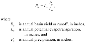 (1)
(1)
The graph relating mean annual temperature and potential evapotranspiration is available in Langbein and others (1949), Langbein (1961), and Chapman and Young (1972). The graph relating Pa/La to Ra/La is available in Langbein (1961) and Chapman and Young (1972). Alternatively, B.A. Contor (Idaho State University, written commun., March 9, 2006) derived a regression equation with a correlation coefficient (R2) of 0.96 describing the relations in the latter graph:
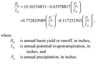 (2)
(2)
At low values of precipitation, this equation calculates runoff values greater than precipitation, thus Contor applied an alternative linear calculation for Pa/La ratios less than 0.55:
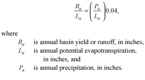 (3)
(3)
As used here, it is assumed that basin yield is equal to ground-water recharge because the sediments that compose the SVRP valley floor are highly permeable, and little surface drainage reaches the Spokane and Little Spokane Rivers. An important limitation of the method is that it is applicable only to annual time periods. To calculate values for shorter time increments, annual values must be divided by some scheme such as simple division.
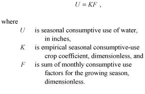
The USDA method is based on the Blaney-Criddle formula (Blaney and Criddle, 1962) for calculating crop consumptive use:
 (4)
(4)
Equation 4 is then restated for monthly consumptive use as:
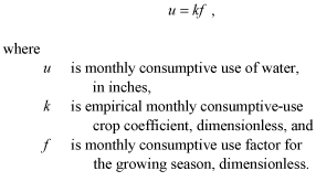 (5)
(5)
The monthly consumptive use factor(f) is calculated with equation 6:
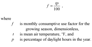 (6)
(6)
Representative values for K and k are given in Blaney and Criddle (1962).
In order to refine the calculation of the consumptive use crop coefficient (k) for application to shorter time periods with more climatic variability, U.S. Department of Agriculture (1970) describes a modification of the Blaney-Criddle formula where k is calculated by:
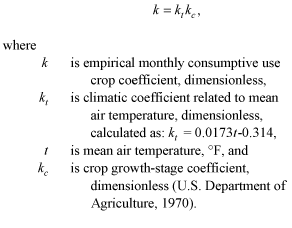 (7)
(7)
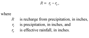
To calculate consumptive use, effective rainfall must be known, defined as the amount of precipitation that is available for crop consumptive use. The equation given in U.S. Department of Agriculture (1970) for effective rainfall is:
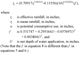 (8)
(8)
Potential consumptive use (u) can be taken as either potential evapotranspiration or calculated with equations 5, 6, and 7, yielding:
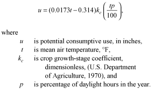 (9)
(9)
Values for rt, t, and p can be specified for annual, monthly, or shorter time periods. If the calculated effective rainfall (re) exceeds either the mean rainfall (rt) or mean consumptive use (u), it must be set to the lower of the latter two values.
In their transient ground-water flow model of the Spokane Valley, Bolke and Vaccaro (1981) used the USDA method to determine effective rainfall and assumed that effective rainfall was equal to actual evapotranspiration, thus yielding equation 10, the amount of recharge from precipitation:
 (10)
(10)
Bolke and Vaccaro (1981) further assumed mean monthly consumptive use (u) was equal to potential evapotranspiration at Spokane.
In preparing data sets for the SVRP aquifer model, B.A. Contor (written commun., March 9, 2006) determined that for low values of precipitation, effective precipitation can be negative as a result of using values lower than those used to develop the non-linear regression. Consequently, for precipitation amounts less than 0.96 in., he developed equation 11 to calculate effective precipitation (re):
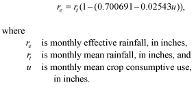 (11)
(11)
The central assumption in applying this method to determination of recharge is that any precipitation not necessary for plant growth (evapotranspiration) is recharged to ground water.
As part of the Eastern Snake Plain Aquifer Model Enhancement Project (ESPAM), a geographic information system (GIS)-based method was developed to calculate recharge based on the PRISM gridded maps of monthly precipitation (Daly and others, 1994, 1997, 1998) and generalized soil maps (Contor, 2004; Cosgrove and others, 2006). The calculations are based on earlier work by Rich (1951, 1952), who measured water yield from basins with forest and rangeland vegetation in the Sierra Ancha experimental forest in central Arizona. Rich (1951, 1952) plotted runoff against precipitation for several watersheds to produce a separate curve for each basin. Contor (2004) fit equations to these curves yielding:
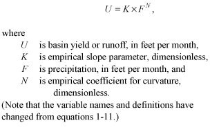 (12)
(12)
Contor (2004) further modified Rich’s method in several ways in order to apply it to the shorter time periods and geologic conditions required by the ESPAM model. Like the SVRP aquifer area, most of the eastern Snake River Plain (ESRP) has little surface-water drainage that reaches the main through-flowing river, and Contor assumed that basin yield was equal to recharge. Thus:
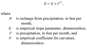 (13)
(13)
This relation is based on the assumption that a plot of recharge against precipitation has a low slope until sufficient precipitation occurs to exceed the requirements of soil-moisture storage, ponding, evaporation, and transpiration, after which recharge occurs. At higher values of precipitation, the curve would become linear and approach a slope of 1 (however, although Rich’s (1951, 1952) data were collected over 15 years, with one year exceeding 200 percent of the mean precipitation, annual precipitation was still insufficient to reach this threshold). The distance the recharge curve is offset from the 1:1 line is controlled by the potential for precipitation to be diverted to the other pre-recharge precipitation requirements mentioned above. The degree of curvature in the early, exponential part of the curve is controlled by preferential recharge pathways within the soil profile, and any surface concentration of precipitation due to topography. The application of the method to shorter time periods changes the relative importance of each of these other pre-recharge requirements; thus the equation parameters are dependent on the time-step length selected and also are unit-dependent. Contor (2004) used annual recharge values and generalized soil types from a previous ESRP ground-water flow model (Garabedian, 1992) to develop monthly parameters for three different soil types: lava rock (K=0.69, N=1.2), thin soil (K=0.463, N=1.5), and thick soil (K=0.136, N=2), where the units are in feet per month. These parameters were calibrated to match annual volumes of recharge used in the previous modeling effort by Garabedian (1992) as well as to match the curvature and transition points suggested by theoretical monthly values of pre-recharge precipitation requirements for each of the three soil types. Garabedian (1992), in turn, based his annual recharge values on those of Mundorff and others (1964), who used a simple precipitation to water-yield ratio derived from eight basins draining to the ESRP.
Because recharge cannot exceed precipitation, the slope of the recharge-precipitation line cannot exceed one. Low values of precipitation must first satisfy the pre-recharge requirements of soil-moisture storage, ponding, evaporation, and transpiration before recharge can occur, resulting in a nonlinear recharge curve. With increasing precipitation, these pre-recharge requirements are satisfied, the curve becomes linear, and there is a one-to-one linear relation between additional precipitation and additional recharge. To automate the calculation of recharge values, Contor derived the transition point—the point where the line makes the transition from exponential to linear and the non-linear function reaches a slope of one—defined as:
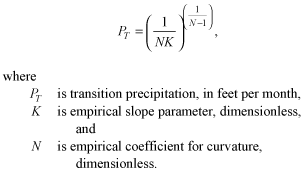 (14)
(14)
Thus, for precipitation amounts less than the transition precipitation (PT), equation 13 is used to determine recharge; for amounts greater than PT, equation 15 is used:
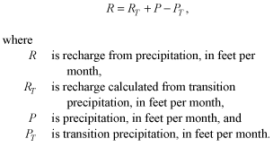 (15)
(15)
Contor (2004) further modified Rich’s approach by cumulatively applying precipitation for November through February as if it all occurred in February. This procedure was followed because winter-time recharge is increased owing to decreased evapotranspiration and temporal concentration of recharge resulting from episodic snow accumulation and melting. This adjustment implies that all snowfall accumulates until a single February thaw event. While this would be unrealistic in the SVRP aquifer area where thaw events are more frequent than in the ESRP, reduced evapotranspiration and episodic snow and melting events would still occur. To address these processes but to avoid applying all winter recharge in February, Contor proposed multiplying winter precipitation by four before recharge is calculated and then dividing the calculated recharge by four, resulting in precipitation/recharge ratios that are less affected by the pre-recharge factors and thus increasing recharge (B.A. Contor, written commun., September 11, 2006).
Another approach to the determination of recharge is to calculate actual (versus potential) evapotranspiration (accounting for processes such as soil-moisture storage and direct evaporation) and determine the amount of precipitation that passes through the root zone (and thus becomes recharge). The difficulty lies with determination of actual evapotranspiration without extensive field measurements.
Due to shortcomings in other methods for estimating reference evapotranspiration, including the earlier Blaney-Criddle FAO method, the FAO developed an approach dubbed the FAO Penman-Monteith equation (Allen and others, 1998). The reference evapotranspiration calculated with this newer equation is then used with crop evapotranspiration coefficients to estimate crop-water requirements. The FAO Penman-Monteith equation for calculating reference evapotranspiration is:
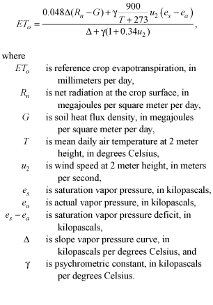 (16)
(16)
One of the characteristics of the FAO Penman-Monteith approach is an emphasis on applicability. Because most of these parameters are not commonly measured, Allen and others (1998) devoted a chapter in their paper to their calculation with commonly available meteorological data.
To calculate crop consumptive use (under standard conditions), the reference evapotranspiration (ETo) is multiplied by a crop coefficient (Kc):
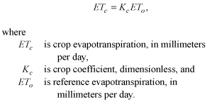 (17)
(17)
The crop coefficient (Kc) for specific crops may be calculated using procedures described in Allen and others (1998). To refine crop-water requirement estimates, these calculations account for growth stage. Alternatively, typical values for Kc are available in the literature. It is important to note that Kc values usually are given for either a grass or alfalfa reference crop; the coefficients given in Allen and others (1998) are for grass. To convert alfalfa-referenced Kc values to grass-referenced Kc values, Kc is multiplied by a factor ranging from 1.0 to 1.3, depending on climate. For Kimberly, Idaho (in south-central Idaho), the conversion factor is 1.24 (Allen and others, 1998).
In this report, the initial attempt to use the FAO Penman-Monteith method to determine recharge simply subtracts crop evapotranspiration (ETc) from precipitation. This approach is hereafter referred to as the single-coefficient FAO Penman-Monteith method.
The FAO Penman-Monteith method can be carried a step further by splitting the crop coefficient (Kc) into two components: the basal crop coefficient (Kcb), which accounts for crop transpiration, and the soil evaporation coefficient (Ke). This calculation of dual-crop evapotranspiration (ETcd) allows estimation of the effects of specific wetting events on Kcand was intended for daily calculation of irrigation requirements. The equation for dual-crop evapotranspiration is:
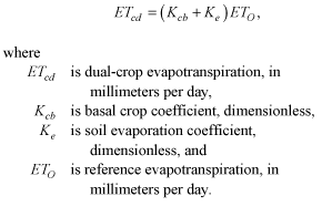 (18)
(18)
The basal crop coefficient (Kcb) for specific crops is available in Allen and others (1998) or in other literature. The soil evaporation coefficient is calculated using constants and procedures described in Allen and others (1998).
Deep percolation from the soil zone can be calculated by a simple mass-balance approach that assumes deep percolation is equal to recharge. Thus, this equation yields recharge for the dual-coefficient FAO Penman-Monteith method:
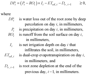 (19)
(19)
Further adjustments to crop consumptive use for non-standard conditions can be made to account for environmental stresses and constraints on crop growth such as pests, soil salinity, water-logging, or drought. These techniques are not considered in this report because they cannot be reliably applied over a large area.

![]() U.S.
Department of the Interior | U.S. Geological
Survey
U.S.
Department of the Interior | U.S. Geological
Survey
Persistent URL: https://pubs.water.usgs.gov/sir20075038
Page Contact Information: Publications Team
Page Last Modified: Thursday, 01-Dec-2016 19:41:27 EST
