Scientific Investigations Report 2007–5044
U.S. GEOLOGICAL SURVEY
Scientific Investigations Report 2007–5044
The geologic history and the hydrogeologic framework of the SVRP aquifer are presented in the reports by Kahle and others (2005) and Kahle and Bartolino (2007). The following discussion briefly summarizes the geologic setting of the study area. The remainder of the discussion focuses on the hydrologic information used to develop the ground-water flow model. Topics covered include the areal and vertical extent of the aquifer, hydraulic properties, inflows and outflows, interaction between the aquifer and the Spokane River, and ground-water levels and movement.
Kahle and Bartolino (2007) described three distinct hydrogeologic units in the study area: the SVRP aquifer, the Basalt and fine-grained interbeds unit, and the Bedrock unit. Together, the Basalt and fine-grained interbeds unit, which includes Columbia River basalt and interbedded lacustrine deposits of the Latah Formation, and the Bedrock unit, which includes Precambrian to Tertiary metamorphic and intrusive igneous rocks, laterally bound and underlie the SVRP aquifer.
The SVRP aquifer consists mostly of sands, gravels, cobbles, and boulders primarily deposited by a series of catastrophic glacial outburst floods from ancient glacial Lake Missoula during the Pleistocene Epoch. Kahle and Bartolino (2007) noted that most of the aquifer sediments deposited in such a high-energy depositional environment are coarse grained. However, they also noted that fine-grained layers of clay and silt are scattered throughout the aquifer and likely were deposited in large proglacial lakes in the path of the Missoula floods. From analysis of drillers’ reports, Kahle and Bartolino (2007) found that
“The aquifer generally has a greater percentage of finer material near the margins of the valley and becomes more coarse and bouldery near the center throughout the Rathdrum Prairie and Spokane Valley. In the Hillyard Trough, the deposits generally are finer grained and the aquifer consists of sand with some gravel, silt, and boulders.”
The areal extent of the SVRP aquifer has been redefined several times in the past 30 years. The most recent definition is the 2005 revised extent of the SVRP aquifer shown in Kahle and others (2005, pl. 2). In most places, the aquifer boundary follows the contact between the coarse, highly permeable aquifer sediments and the surrounding less permeable bedrock and fine-grained material. The 2005 revised extent includes Ramsey Channel, Chilco Channel, the south part of Hoodoo Valley, and the south part of Cocolalla Valley (fig. 1). These four areas lie outside the Sole Source Aquifer as designated by the U.S. Environmental Protection Agency in 1978. In revising the aquifer boundary, Kahle and others (2005, p. 17) noted that
“For modeling purposes, it may be important to use a more inclusive aquifer boundary to better represent contributions from adjacent surficial deposits that are in hydraulic contact with the Sole Source Aquifer.”
For the most part, the extent of the model in this report coincides with the 2005 revised extent. However, the model excludes Spirit and Hoodoo Valleys and three areas where bedrock is close to land surface and the aquifer sediments likely are unsaturated (fig. 1). The model extent is not intended to be a redefinition of the aquifer. As discussed in the following paragraphs, Spirit and Hoodoo Valleys are excluded from the model because of uncertainties about the ground-water flow directions in those valleys and the degree of hydraulic connection between the valleys and northern Rathdrum Prairie.
The 2005 revised extent of the SVRP aquifer extends into the west part of Spirit Valley and the south part of Hoodoo Valley (fig. 2). Kahle and others (2005, p. 20) stated that
“In the Hoodoo Valley, historical water-level elevations indicated that a water-table divide was between Edgemere and Harlem (Walker, 1964). Ground water north of the divide moved northward toward the Pend Oreille River; ground water south of the divide moved southward toward Athol. In Spirit Valley, the ground-water divide was near Blanchard Lake (Parliman and others, 1980). West of the divide, ground water flows northwestward toward the Pend Oreille River; east of the divide, ground water flows southeastward into the main body of the SVRP aquifer.”
An examination of recent water-level data and drillers’ reports indicates that the previous characterization is subject to uncertainty. During the synoptic water-level measurements of September 2004 (Campbell, 2005), water levels in wells 262 and 263, at the south end of Hoodoo Valley, were several feet higher than water levels in wells 260 and 261, which are farther to the north (fig. 2, table 1). These water levels indicate that ground water flows to the north (away from northern Rathdrum Prairie) in almost the entire length of Hoodoo Valley. In Spirit Valley, water levels were measured at only one well (well 267) during September 2004. However, a search of the USGS ground-water database produced several water-level measurements for wells in the valley during the late summer of 1998 and 1999. Water levels in wells S-1, S-2, and 267 (fig. 2, table 1) indicate that the ground water flows away from the Rathdrum Prairie in almost the entire length of Spirit Valley.
The synoptic water-level measurements of September 2004 (Campbell, 2005) also show a water-level difference of about 100 ft over a relatively short distance of about 1 mi from the south end of Hoodoo Valley to northern Rathdrum Prairie. Water levels in wells 262 and 263 were 2,158.17 and 2,151 ft, respectively. Water levels in wells 264 and 266 were 2,044.18 and 2,035.78 ft, respectively. Drillers’ reports for T. 54 N., R. 4 W. and the north half of T. 53 N., R. 4 W. show a similar water-level difference from the south end of Hoodoo Valley to northern Rathdrum Prairie. The relatively large water-level difference over a relatively short distance can indicate the presence of a low hydraulic conductivity barrier resulting in a poor hydraulic connection between Hoodoo Valley and northern Rathdrum Prairie. However, although clay layers are noted in some drillers’ reports for the area, conclusive evidence of a low hydraulic conductivity barrier is lacking.
Considered together, available data indicate uncertainty in ground-water flow directions in Spirit and Hoodoo Valleys and in the degree of hydraulic connection between those valleys and northern Rathdrum Prairie. Because of this uncertainty, the model in this report terminates at boundary segment A-B (fig. 2) and does not extend into Spirit and Hoodoo Valleys. If ground-water inflow from these valleys to northern Rathdrum Prairie does occur, the inflow is assumed to be negligible. During model calibration, the uncertainty in ground-water inflow from Spirit and Hoodoo Valleys is treated by assuming different inflow values along boundary segment A-B.
In addition to Spirit and Hoodoo Valleys, three areas in the 2005 revised extent are excluded from the model (fig. 1). The first excluded area is on the east side of northern Rathdrum Prairie. Hydrogeologic sections L-L’ and O-O’ in Kahle and Bartolino (2007, pl. 2) indicate that bedrock is close to land surface in this area and the aquifer sediments likely are unsaturated. The second and third excluded areas are two narrow zones that border Five Mile Prairie and the subsurface bedrock ridge that extends from the prairie toward the south. The aquifer sediments in the two narrow zones likely also are unsaturated as they lie on the slope of the basalt that outcrops to form Five Mile Prairie.
The sediments of the SVRP aquifer extend from land surface downward to either bedrock or the Latah Formation, which is composed predominantly of lacustrine and fluvial deposits of siltstone, claystone, and minor sandstone. The altitude of the base of the aquifer as determined by Kahle and Bartolino (2007) is shown in figure 3. Sediment thickness (from land surface to the base of the aquifer) is largest in the central part of the aquifer and thins to zero at the aquifer perimeter. The maximum sediment thickness is about 800 ft in northern Rathdrum Prairie, 500 ft near the Washington-Idaho State line, and 700 ft in Hillyard Trough. However, the saturated thickness (from the water table to the base of the aquifer) can be substantially less than the sediment thickness. For example, in northern Rathdrum Prairie, the depth from the land surface to the water table can exceed 500 ft, and the maximum saturated thickness is between 200 and 300 ft. In the area underlain by shallow bedrock (fig. 3) the saturated zone likely is a thin veneer overlying the bedrock or is entirely absent.
The SVRP aquifer is considered to be a single hydrogeologic unit except in Hillyard Trough and the Little Spokane River Arm. In those areas, a continuous clay layer divides the aquifer into an upper unconfined unit and a lower confined unit. Kahle and Bartolino (2007) characterize this clay layer as a “fine-grained layer.” However, the term “clay layer” is used in this report to emphasize the low-permeability character of the layer. The areal extent of the clay layer as mapped by Kahle and Bartolino (2007) is shown in figure 4. The vertical extent of the clay layer is shown in hydrogeologic section C-C’ in figure 5. According to Kahle and Bartolino (2007), the average thickness of the clay layer is 215 ft in Hillyard Trough and 130 ft in the Little Spokane River Arm. In Hillyard Trough, the altitude of the top of the clay layer is between 1,660 and 1,720 ft. In the Little Spokane River Arm, the altitude of the top of the clay layer is between 1,500 and 1,700 ft.
The SVRP aquifer is a highly productive aquifer. Wells in the aquifer yield as much as several thousand gallons per minute with relatively little drawdown. Many wells penetrate only the upper part (less than 100 ft) of the aquifer’s saturated thickness. Kahle and others (2005, p. 19-20) noted that hydraulic conductivity of the aquifer sediments is at the upper end of values measured in the natural environment. However, the aquifer also contains local zones of less permeable, fine-grained sedimentary materials.
Multiple-well aquifer tests, specific-capacity data, and computer model analyses have been used in previous studies to estimate the horizontal hydraulic conductivity (Kh) of the SVRP aquifer. Aquifer tests and specific capacity data are more numerous in more populated regions of the SVRP aquifer—from the city of Spokane, Washington, on the west to Post Falls and Coeur d’Alene, Idaho, on the east. There is significantly less information on hydraulic properties in Rathdrum Prairie north of Post Falls and Coeur d’Alene.
Data for nine multiple-well aquifer tests conducted in the west half of the SVRP aquifer (fig. 6) are given by CH2M Hill (1998, 2000). These data appear to be the only multiple-well aquifer-test data readily available from published sources. Estimated Kh values given in the reports range from 500 to 6,200 ft/d (CH2M Hill, 1998, p. 2-22 and tables 2-7; CH2M Hill, 2000, table E-2). However, analyses of the tests are complicated by the fact that the pumped and observation wells do not penetrate the entire thickness of the aquifer.
Specific capacity is the ratio of pumping rate to drawdown in a well after a given pumping duration. However, there is no commonly accepted pumping duration and it can be highly variable from one test to the next. Consequently, Kh values estimated from specific-capacity data are not as reliable as values estimated from multiple-well aquifer-test data.
Sagstad (1977), Bolke and Vaccaro (1981), and CH2M Hill (1998) estimated Kh from single-well specific capacity data. Bolke and Vaccaro (1981, p. 18) indicated a decrease in Kh values in a westerly direction from the Post Falls area. They stated:
“The decrease in values in the down-valley direction is indicative of the change in valley-fill material, which, in general grades from coarse to fine in a westerly direction.”
The estimated Kh values given by Bolke and Vaccaro (1981) average about 6,000 ft/d in the Post Falls area, about 4,300 ft/d in Spokane Valley, about 2,600 ft/d near Spokane, and about 860 ft/d in Hillyard Trough and the Little Spokane River Arm.
CH2M Hill (1998, p. 2-24 and tables 2-8) indicated that Kh values estimated from analysis of 31 specific capacity tests range from 100 to 6,200 ft/d for the west half of the SVRP aquifer. The central 50 percent of the values range from 400 to 3,000 ft/d. However, CH2M Hill (1998) also noted that
“For many wells, including those closest to the State line, the computed transmissivities [horizontal hydraulic conductivity times saturated thickness] appear to underestimate the likely aquifer transmissivity because the wells pump at low rates or are shallow (for example, they penetrate only a very small fraction of the aquifer’s saturated thickness).”
In a hydrogeologic study of southern Rathdrum Prairie, Sagstad (1977, p. 39-40) analyzed specific-capacity data for 20 wells in the Post Falls area and 4 wells in the Coeur d’Alene area. The estimated Kh values given by Sagstad (1977) range from 250 to 2,100 ft/d in the Post Falls area and from 240 to 900 ft/d in the Coeur d’Alene area. Sagstad noted that
“Transmissive characteristics in the Post Falls area generally are higher than in the Coeur d’Alene area. Well logs show that greater percentages of coarse gravels, pebbles, and sands are present in the Post Falls area than in the Coeur d’Alene area.”
This characterization is consistent with a steeper water-table gradient in the Coeur d’Alene area than in the Post Falls area, as shown by the ground-water level map of Campbell (2005).
Horizontal hydraulic conductivity values used in previous computer models generally were higher than values estimated from multiple-well aquifer tests and specific-capacity data. In the model by Bolke and Vaccaro (1981, p. 20), Kh values ranged from about 1,000 to 11,000 ft/d. These values result from an upward adjustment, by a factor of 1.9, of the initial values estimated from specific-capacity data. In the final model of CH2M Hill (2000, fig. J-4), Kh values ranged from 2,000 ft/d in northern Hillyard Trough to 7,000 ft/d at the Idaho-Washington State line. In the model by Golder Associates, Inc. (2004, fig. 6.8), Kh values ranged from about 260 ft/d in northern Hillyard Trough to about 57,000 ft/d at the Idaho-Washington State line.
The model by Buchanan (2000) is the only previous model that encompasses the entire SVRP aquifer. In that model, on the east side of the aquifer, a zone that has a Kh value of 11,000 ft/d extends from Lake Pend Oreille toward the west through northern Rathdrum Prairie and then toward the south through West Channel into southern Rathdrum Prairie. Lower Kh values (220 ft/d or less) are assigned to areas near the aquifer perimeter and in side valleys. This characterization is consistent with the steeper water-table gradients in side valleys in which Hauser, Hayden, Newman, and Spirit Lakes are located (see water-level map of Campbell, 2005). On the west side of the aquifer, Kh values are similar to those in the CH2M Hill (2000) model.
Considered together, available data indicate that Kh values in the central part of the SVRP aquifer range from about 1,000 ft/d to several tens of thousands of feet per day. In Hillyard Trough and in the vicinity of Coeur d’Alene, Kh values appear to be near the low end of the range. Near the aquifer perimeter and in side valleys, Kh values might be a few hundred feet per day or less.
Few field-measured vertical hydraulic conductivity (Kv) data were available for the SVRP aquifer and for the clay layer that separates the upper and lower aquifer units in Hillyard Trough and the Little Spokane River Arm. In the models by CH2M Hill (1998, 2000) and Golder Associates, Inc. (2004), the ratio of Kh to Kv in the aquifer was assumed to be 10:1 and 3:1, respectively. The report by Golder Associates, Inc. (2003, p. 5-24) refers to an aquifer test conducted near the Colbert Landfill (about 10 mi north of Spokane) where a clay layer separates an upper aquifer from a lower aquifer. Both the clay layer in Hillyard Trough and the clay layer near the Colbert Landfill are believed to have been deposited within a glacial lake environment. Golder Associates, Inc. (2003, p. 5-24) noted that
“During pump tests at wells near the Colbert Landfill (Landau Associates, 1991) no response in the upper sands and gravels was observed during pumping from the lower sands and gravels, indicating that the glacial lake sediments act as a vertical hydraulic barrier between the upper and lower sand and gravel units in this area.”
However, it is uncertain if this characterization also applies to the clay layer in Hillyard Trough and the Little Spokane River Arm.
Few field-measured specific yield (SY) data were available for the SVRP aquifer. In the model by Bolke and Vaccaro (1981), SY values initially were estimated from published tables that relate SY to grain size and subsequently adjusted during model calibration. Values of SY in the calibrated model ranged from about 0.1 to 0.2. In the model by Golder Associates, Inc. (2004, fig. 6-8), a similar procedure yielded SY values that ranged from 0.125 to 0.3. The models by CH2M Hill (1998, 2000) and Buchanan (2000) do not consider SY because those models assume steady-state flow conditions.
Inflows to the SVRP aquifer include (1) recharge from precipitation, (2) inflows from tributary basins and adjacent uplands, (3) subsurface seepage and surface overflows from lakes that border the aquifer, (4) flow from losing segments of the Spokane River to the aquifer, (5) return percolation from irrigation, and (6) effluent from septic systems. For the ground-water flow model in this report, monthly inflows were estimated for October 1990 through September 2005. Areally distributed inflow components, such as recharge from precipitation, are computed on a raster grid with a cell size of 1,320 by 1,320 ft. To facilitate preparation of model input data, the raster grid is aligned with the finite-difference grid used in the model.
Recharge from precipitation refers to that part of precipitation that infiltrates into the subsurface and percolates downward to reach the water table. Precipitation can enter the subsurface by falling on a permeable surface and infiltrating into the ground or falling on an impermeable (paved) surface and running off to a recharge (“dry”) well, an infiltration basin, or an adjacent permeable surface. In both cases, part of the precipitation is consumed by evapotranspiration, either on land surface or as the water percolates through the root zone (typically, the top several feet of subsurface). The water that percolates below the root zone is referred to as deep percolation. The assumption is that evapotranspiration does not occur below the root zone, and water that becomes deep percolation eventually reaches the water table.
If precipitation falls on a permeable surface within the SVRP aquifer, the entire amount of precipitation is assumed to enter the ground and there is no overland runoff. This assumption is reasonable for the SVRP aquifer because the aquifer material is highly permeable. The monthly rate of deep percolation resulting from precipitation on a permeable surface is denoted by DP and is expressed in units of length over time—for example, inches per month.
To estimate DP, the FAO Penman-Monteith method developed by Allen and others (1998) was used to estimate evapotranspiration. Bartolino (2007) used the method to estimate daily evapotranspiration for 1990–2005 at six weather stations in the vicinity of the model area (fig. 7). Daily deep percolation at each weather station was determined from a daily soil-moisture balance calculation (Bartolino, 2007, p. 11, eq. 19). The daily deep percolation values then were aggregated over each month to determine the DP value for each weather station.
The areal distribution of DP is estimated by linearly interpolating the DP values for the six weather stations. To perform the interpolation, an initial triangular network is constructed using the six weather stations as vertices. However, this initial network does not encompass the full extent of the model. Therefore, three auxiliary vertices are added to expand the network (fig. 7). The DP at an auxiliary vertex is set equal to the DP at the closest weather station. For any point within the expanded network, DP is interpolated linearly from the DP values for the three vertices of the triangle containing the point.
If precipitation falls on an impermeable surface and then runs off to a recharge well, an infiltration basin, or an adjacent permeable surface, the assumption is that 15 percent of the runoff is consumed by evapotranspiration and the remaining 85 percent becomes deep percolation. Because infiltration is focused into the recharge well, infiltration basin, or along the edges of the adjacent permeable surface, loss to evapotranspiration probably is relatively low. The monthly rate of deep percolation resulting from precipitation on an impermeable surface is denoted by DI.
Two data sets are used to estimate the areal distribution of DI. The first contains values for the amount of impermeable surface in the model area, and the second contains values for precipitation throughout the model area. The amount of impermeable surface is estimated from aerial photographs and National Land-Cover Data (http://erg.usgs.gov/isb/pubs/factsheets/fs10800.html) for four periods: 1990–95, 1996–99, 2000–02, and 2002–05. Within each period, the amount of impermeable surface is assumed to remain constant in time. Precipitation throughout the model area is obtained from PRISM-derived data. PRISM is an acronym for “Parameter-elevation Regressions on Independent Slopes Model” and was developed by the Oregon Climate Service of Oregon State University (http://www.ocs.orst.edu/prism/products/). PRISM uses point data, a digital elevation model, and other spatial data sets to generate gridded estimates of several spatial and temporal climatic parameters, including precipitation.
The areal distribution of DI is calculated on a raster grid with a cell size of 1,320 by 1,320 ft. For each cell in the grid, DI is calculated as
DI = P × fI × 0.85, (1)
where
| P | is the monthly precipitation rate, and |
| fI | is the fraction of the cell’s surface area that is impermeable. |
Runoff from impermeable surfaces in certain parts of Spokane and Coeur d’Alene where the runoff is routed into a sewer overflow system that discharges to the Spokane River was excluded from the calculation.
Combining DP and DI, the monthly rate of deep percolation (D) at a cell is calculated as
D = (1 – fI) DP + DI . (2)
Note that for any given month, D is the downward flux at the base of the root zone. This downward infiltration must travel through the unsaturated zone to reach the water table. According to unsaturated flow theory, the transmission time of an infiltration front to a given depth depends on the prevailing moisture conditions in the unsaturated zone. In this study, a simple approximation is adopted in which the traveltime to the water table is linearly related to the depth of the water table.
To estimate the transmission time to the water table, water levels recorded at well 251 are compared to the monthly rates of deep percolation (D) for the well site (fig. 8). Well 251 is selected for analysis because the water level in the well is about 400 ft below land surface and the well has a long period of record. For each water year during which the hydrograph peak and trough are not masked by the long-term trend, the point of steepest water-level rise, assumed to be approximately halfway between the trough and the peak, is indicated by a triangle on the graph. The time of steepest water-level rise is assumed to correspond to the time of greatest recharge at the water table. The steepest water level rise typically occurs around May (fig. 8). However, deep percolation at the base of the root zone is greatest around the preceding December or early January. This observation indicates a transmission time of about 5 months is needed for precipitation infiltration to reach the water table at a depth of about 400 ft. The estimated transmission time to reach the water table at different depths, based on linearly prorating the transmission time to the depth of 400 ft, is shown in table 2.
The monthly volumetric rate of recharge (in cubic feet per second) from precipitation to the (1) Idaho side of the SVRP aquifer model, (2) Washington side of the model, and (3) entire model is shown in figure 9. The volumetric rate of recharge from precipitation is lower on the Washington side than on the Idaho side. Also, the recharge peaks earlier on the Washington side than on the Idaho side, because the water table generally is at a shallower depth on the Washington side than on the Idaho side.
The average volumetric rate of recharge and the average recharge flux from October 1990 through September 2005 is shown in table 3. For the entire model, the average volumetric rate of recharge from precipitation is 228 ft3/s. The average volumetric rate of recharge on the Idaho side of the model is about twice that on the Washington side. The average recharge flux is calculated as the average volumetric rate divided by the surface area. Although precipitation generally is higher on the Idaho side of the model than on the Washington side, the recharge flux is about the same on both sides. This is because a higher percentage of precipitation enters the subsurface through recharge wells and infiltration basins on the Washington side than on the Idaho side. Infiltration through recharge wells and infiltration basins generally is subject to less evapotranspiration loss than infiltration through permeable surfaces.
The SVRP aquifer receives flow from higher altitude regions immediately adjacent to the aquifer. These regions are referred to as tributary basins and adjacent uplands or simply as tributary basins. A tributary basin might drain directly into the aquifer or drain into a lake that, in turn, recharges the aquifer. Tributary basins that drain directly to the aquifer are shown in figure 10. Recharge from these basins to the aquifer is estimated in this section of the report. Tributary basins that drain into seven of the nine lakes that border the aquifer are shown in figure 10—Lake Pend Oreille and Coeur d’Alene Lake are not included. Recharge from the lakes to the aquifer is estimated in section, “Lakebed Seepage and Surface Overflows.”
Flow from tributary basins to the SVRP aquifer is estimated using regional regression equations developed by Hortness and Berenbrock (2001). These regression equations are developed for Idaho and parts of adjacent States to estimate the mean annual discharge at ungaged sites on streams that are unaffected by regulations and (or) diversions. The methodology uses the USGS StreamStats web application (Ries and others, 2004) and the ArcGIS-ArcHydro application developed by Environmental Systems Research Institute, Inc. Both tools make use of the same techniques and underlying data sets. In the following discussion, this methodology is referred to as StreamStats. The estimation of tributary basin discharge to the aquifer was performed by Jon Hortness and is included in the report by Kahle and Bartolino (2007).
The regression equations in StreamStats are developed by relating the mean annual discharge values for long-term gaging stations to various physical and climatic characteristics (basin characteristics) of the upstream drainage basin. For a gaged site, the mean annual discharge is the average of all annual discharges in the data record or during a specific period of years. For an ungaged site, the estimated mean annual discharge is a long-term average for a time period that is comparable to the length of record used to develop the regression equations. Typically, the data record spans tens of years.
To apply StreamStats, 72 tributary basin outlet points are selected along the model boundary (fig. 10). For each outlet point, the upstream drainage basin is delineated. The combination of all delineated basins encompasses most of the surrounding uplands that drain into the SVRP aquifer. Small gaps between adjacent basins are not included. For each delineated basin, StreamStats is used to estimate the mean annual discharge at the outlet point. Because bedrock occurs either at the basin surface or under a thin layer of soil, the assumption is that minimal subsurface discharge occurs at the outlet. Therefore, stream discharge accounts for nearly all discharge from the basin. However, as the stream crosses from the tributary basin onto the aquifer, all stream water quickly soaks into the ground because of the highly permeable nature of the aquifer material.
The 72 tributary basins range in area from 0.3 to 24 mi2. The estimated mean annual discharge ranges from 0.0037 to 15 ft3/s, and the sum of the mean annual discharges of all 72 tributary basins is 112 ft3/s. StreamStats also provides error statistics on the estimated discharge values. Typically, the 67-percent confidence interval ranges from 0.4 to 1.6 times the estimated value. An assessment of the StreamStats estimates is included in the section, “Lakebed Seepage and Surface Overflow.”
The mean annual discharge estimated by StreamStats is the long-term average flow from a tributary basin to the SVRP aquifer. For a particular month, the flow from the tributary basin is higher or lower than the long-term average value. To allow for temporal (monthly) variability in flow, a scaling index is used to convert the long-term average flow into the flow for a particular month. In this study, monthly flow on the Little Spokane River at the gaging station at Dartford, Washington, is assumed to be an appropriate scaling index. Because the tributary basins that drain to the Little Spokane River are in close proximity to the tributary basins that drain to the aquifer, these two sets of basins likely share similar physical and climatic characteristics.
The monthly flow from a tributary basin to the SVRP aquifer is estimated as
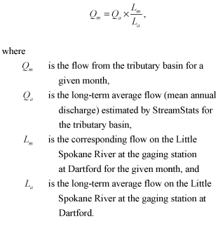 (3)
(3)
The scaling index (Lm / La) for each month from October 1990 to September 2005 is shown in figure 11. The long-term average flow at the gaging station at Dartford is computed using discharge data for 1960–2000.
The SVRP aquifer is recharged by lakes that border the aquifer. Of the nine lakes along the perimeter of the model area, only the two largest lakes (Lake Pend Oreille and Coeur d’Alene Lake) have perennial outlet streams. For the seven smaller lakes, outflow occurs as subsurface seepage through the lakebed and occasional surface overflow when the lake level rises above the outlet structure. Because of the highly permeable nature of the aquifer material, the surface overflow soaks into the ground within a short distance of the lake. Therefore, the combined outflow from subsurface lakebed seepage and surface overflow is the amount of recharge from the seven smaller lakes to the aquifer.
In principle, the outflow from a lake can be estimated by the following water-balance equation:
OL = IL + PL – EL – SL, (4)
where
| OL | is rate of outflow from the lake, |
| IL | is the rate of inflow to the lake from the surrounding tributary basins, |
| PL | is the rate of direct precipitation on the lake surface, |
| EL | is the rate of evaporation from the lake, and |
| SL | is the rate of change in storage in the lake. |
Murray (2007) evaluated the terms on the right-hand side of equation 4 for Hayden Lake on a monthly basis from 1998 through 2005. She noted that PL – EL – SL typically is a small percentage of IL. Therefore, monthly outflow from the lake can be approximated reasonably by the monthly inflow from surrounding tributary basins. This approximation is assumed to be applicable to the seven smaller lakes along the perimeter of the model area (that is, excluding Lake Pend Oreille and Coeur d’Alene Lake).
Murray (2007) estimated inflows to the seven lakes using the same procedure as that used to estimate flow from tributary basins to the SVRP aquifer. For each lake, outlet points are placed along the lake perimeter. For each outlet point, the upstream tributary basin is delineated (fig. 10) and StreamStats is used to estimate the mean annual discharge. The sum of the mean annual discharges for the surrounding tributary basins is the long-term average inflow to the lake (table 4). Finally, the monthly inflow to the lake is estimated by multiplying the long-term average inflow by the scaling index (Lm / La) in the same manner as that used to estimate monthly flow from a tributary basin to the aquifer (eq. 3). Assuming monthly inflow to the lake equals monthly outflow from the lake, the long-term average inflow to the lake times the scaling index is the monthly flow from the lake to the aquifer.
An assessment of the StreamStats methodology can be made by comparing the StreamStats estimates with basin water yields calculated by previous investigators. Pluhowski and Thomas (1968) estimated the water yield of the Rathdrum Prairie Basin, defined as all areas upstream of a north-northwest to south-southeast line drawn at the gaging station on the Spokane River near Otis Orchards (see line O-O’ in fig. 10). For this basin, they estimated a water yield of 530 ft3/s. When expressed in terms of the flow components used in this study, this basin water yield represents the sum of (1) recharge from precipitation to that part of the SVRP aquifer upstream of line O-O’, (2) inflows from all tributary basins to that part of the aquifer upstream of line O-O’, and (3) inflows to the aquifer from Fernan, Hauser, Hayden, Newman, Spirit, and Twin Lakes. The second and third items are estimated by StreamStats. For the period of study (1990–2005), the average values of the three items are 165, 86, and 294 ft3/s, respectively, which sum to 545 ft3/s. Although this sum is somewhat higher than Pluhowski and Thomas’s (1968) basin water yield of 530 ft3/s, especially because Pluhowski and Thomas’s Rathdrum Prairie Basin includes Spirit Valley, which is excluded from the model extent in this study, the comparison does indicate that the StreamStats estimates used in this study are consistent with basin water yields calculated by previous investigators.
For Lake Pend Oreille and Coeur d’Alene Lake, a large part of the lake inflow is discharged to the outlet stream. By comparison, lakebed seepage is a relatively small quantity. Therefore, estimating lakebed seepage by a water-balance calculation for the lake might lead to results that are highly uncertain. Nonetheless, previous investigators have made water-balance calculations for Coeur d’Alene Lake. Seepage from Coeur d’Alene Lake often is estimated in combination with seepage from the segment of the Spokane River upstream of the gaging station near Post Falls. In a study of ground-water inflow to the Rathdrum Prairie, Anderson (1951, p. 20-21) stated that
“Some ground water is believed to be derived from Coeur d’Alene Lake (and the Spokane River between the lake and Post Falls). Approximately three-fourths of the inflow to the lake is gaged and a comparison of estimated total inflow with total surface outflow plus evaporation indicates a seepage loss of about 300 second-feet to ground water.”
However, given that the mean annual flow measured at the gaging station near Post Falls for 1913–2001 is about 6,200 ft3/s (Kahle and others, 2005, p. 41), the calculated seepage loss of 300 ft3/s would be within the error in the discharge measurements and is therefore highly uncertain.
Sagstad (1977) applied Darcy’s Law to estimate recharge to the SVRP aquifer from Coeur d’Alene Lake and from the segment of the Spokane River upstream of the gaging station near Post Falls. The Darcy’s Law calculation was performed for three sections, with flow across section C-C’ (Sagstad 1977, fig. 13 and table 7) approximately representing seepage from Coeur d’Alene Lake. Using a hydraulic conductivity of 535 ft/d, a saturated thickness of 150 ft, and a water-table gradient of 0.00303, the flow across section C-C’ was calculated to be 37 ft3/s.
For Lake Pend Oreille, Pluhowski and Thomas (1968) estimated lakebed seepage by a water-balance calculation for the east (mostly Idaho) part of the SVRP aquifer. Their seepage estimate for Lake Pend Oreille is 50 ft3/s. However, they noted that because of uncertainties in various flow components, “the actual contribution to the aquifer from Pend Oreille Lake may be as much as 200 cfs.”
Losing segments of the Spokane River occur where the stream level is higher than the hydraulic head in the aquifer directly under the streambed. Along a losing segment, water seeps from the stream and recharges the aquifer. Consequently, there is less streamflow at the downstream end of a losing segment than at the upstream end of the segment. The amount of flow from the Spokane River to the SVRP aquifer is discussed in the section, “Interaction between Aquifer and Spokane River.”
Return percolation from irrigation refers to that part of applied irrigation water that is not consumed by evapotranspiration but instead percolates downward past the root zone and eventually reaches the water table. Irrigation includes landscape irrigation (such as lawn watering), agricultural irrigation, and golf course irrigation. For the period of study (1990–2005), nearly all irrigation water applied within the model area is derived from ground-water pumpage. Therefore, return percolation from irrigation actually is water that came from the aquifer.
To estimate water use for landscape irrigation, monthly ground-water withdrawals by water purveyors and by domestic users outside water purveyor service areas is divided into an indoor-use component and an outdoor-use component. For each year, during January, February, March, November, and December, the outdoor-use component is assumed to be zero. Therefore, ground-water withdrawal during those 5 months is entirely for indoor use. For April through October, the indoor-use component is assumed to be the average withdrawal during the aforementioned 5 months with no outdoor use. The outdoor-use component is any withdrawal in excess of the indoor-use component. The entire outdoor-use component is assumed to be for landscape irrigation. Based on studies by Oad and others (1997) and Dukes and others (2005), landscape irrigation efficiency is estimated to be 60 percent. Therefore, 40 percent of the outdoor-use component percolates back to the aquifer.
In a water purveyor service area, ground water is pumped from supply wells and distributed to users in the service area. Water purveyor service areas are delineated for four periods: 1990–95, 1996–99, 2000–02, and 2003–05. Within each period, service areas are assumed to remain unchanged. Water purveyor service areas during 2000–02 are shown in figure 12. For each service area, return percolation is computed from pumpage records for supply wells in the entire service area (see section, “Withdrawals from Wells”) and then distributed uniformly over the service area. For the City of Spokane, however, the service area southwest of the city (fig. 12) is excluded from the return percolation calculation as that area is relatively undeveloped and landscape irrigation is expected to be minimal. Outside water purveyor service areas, ground-water withdrawals are estimated on a cell-by-cell basis on a raster grid (see section, “Withdrawals from Wells”). Return percolation is applied to the same cell from which ground water is withdrawn.
For agricultural irrigation outside water purveyor service areas and for self-supplied golf courses, ground-water withdrawals are estimated from crop acreage, irrigation demand, and an assumed irrigation efficiency of 60 percent. Therefore, 40 percent of the pumped water is assumed to percolate back to the aquifer.
The monthly rate of return percolation from all types of irrigation for the entire model area is shown in figure 13. From October 1990 through September 2005, the average rate of return percolation from irrigation is 54 ft3/s for the entire model area.
For a water user who discharges to a septic system, 95 percent of the indoor use is assumed to become effluent from septic systems that percolates back to the aquifer. For a water user who discharges to a sewer system, the assumption is that none of the indoor use returns to the aquifer. To determine the areal distribution of effluent from septic systems, a raster of sewer hookup density is constructed for each year from 1990 to 2005 using spatial data of city limits, sewer district boundaries, and density of sewer hook-ups within each sewer district. The sewer hookup density raster for 2000 is shown in figure 14. For each cell in the raster, the sewer hookup density is the fraction of homes in the cell that are connected to a public sewer system. If the sewer hookup density is zero, the cell is not in a sewer district and all homes in the cell discharge to septic systems. In this case, 95 percent of the indoor water use within the cell is returned to the aquifer. If the sewer hookup density is 1, then the cell is within a sewer district and all homes in the cell discharge to a sewer system. In this case, none of the indoor water use within the cell is returned to the aquifer. If the sewer hookup density is greater than zero but less than 1, then either the cell is partially within a sewer district or the cell is entirely within a sewer district but not all homes in the cell discharge to the sewer system. In this case, effluent from the septic system is 0.95 (1 – ds) times the indoor water use in the cell, where ds is the sewer hookup density.
The monthly rate of effluent from septic systems for the entire model area is shown in figure 13. The gradually declining rate is caused by expansion of sewer districts. From October 1990 through September 2005, the average rate of effluent from septic systems is 23 ft3/s for the entire model area.
Outflows from the SVRP aquifer include (1) ground-water withdrawals from wells, (2) ground-water discharge from the aquifer to gaining segments of the Spokane River, (3) ground-water discharge from the aquifer to the Little Spokane River, and (4) subsurface outflow at the western limit of the model area near Long Lake. For the ground-water flow model in this report, monthly outflows were estimated for October 1990 through September 2005. Areally distributed outflow components were computed on a raster grid with a cell size of 1,320 by 1,320 ft that was aligned with the finite-difference grid used in the model.
Withdrawals of ground water from the SVRP aquifer were estimated for four categories: (1) withdrawals by water purveyors, (2) withdrawals by domestic users outside water purveyor service areas, (3) withdrawals for agricultural irrigation outside water purveyor service areas and by self-supplied golf courses, and (4) withdrawals by self-supplied industries. The combined monthly withdrawal rate for all four categories is shown in figure 15. From October 1990 through September 2005, the average combined withdrawal rate is 317 ft3/s. Individual withdrawal rates for each category are discussed in the following paragraphs.
Data on withdrawals by water purveyors were obtained from 21 water purveyors in the model area for 1990–2005. This work was performed in conjunction with ongoing USGS water-use data collection (Molly Maupin, U.S. Geological Survey, written commun., 2006). The areal distribution of 159 water purveyor wells is shown in figure 12. Monthly withdrawals were obtained for 125 of the 159 wells, and annual withdrawals were obtained for the other 34 wells. For wells with annual withdrawal data, monthly withdrawals are estimated by distributing the annual withdrawal to each month on the basis of the monthly pumping pattern of other wells operated by the same water purveyor or by another water purveyor serving a similar community. The estimated monthly withdrawal rate by all water purveyors is shown in figure 15. From October 1990 through September 2005, the average withdrawal rate for this category is 205 ft3/s.
Data on withdrawals by domestic users outside water purveyor service areas were not available. Monthly withdrawals were assumed to be similar to the average monthly withdrawals for a water purveyor-supplied home in Spokane. The estimated monthly withdrawal rate for a home outside water purveyor service areas is shown in figure 16. A study by the City of Spokane estimated the rate of indoor use for a home is 25.4 ft3/d (L. Brewer, oral commun., 2006). This indoor use rate is assumed to apply year round for a home outside water purveyor service areas. From April through October, an outdoor-use rate (for landscape irrigation) is added to the indoor-use rate. The outdoor-use rate is based on the outdoor-use pattern for Spokane.
To estimate the areal distribution of withdrawals by domestic users outside water purveyor service areas, the density of homes outside those areas was estimated on a raster grid. The number of homes in each cell was estimated from land-cover data and aerial photographs. The monthly withdrawal rate in each cell was computed as the number of homes in the cell times the monthly withdrawal rate of a home (fig. 16). The estimated monthly withdrawal rate for all homes outside water purveyor service areas is shown in figure 15. From October 1990 through September 2005, the average withdrawal rate for this category is 28 ft3/s.
Withdrawals for agricultural irrigation outside water purveyor service areas and by self-supplied golf courses were estimated from irrigation acreages and irrigation demand. Nearly all withdrawals in this category were on the Idaho side of the SVRP aquifer. Irrigation acreages were estimated from Idaho water rights data and by inspection of aerial photographs. Irrigation acreages are shown on a raster grid of irrigation density in figure 17. For each cell in the raster, the irrigation density is the percentage of the cell’s area that is irrigated. If the irrigation density is 1, all of the cell’s area is irrigated. Conversely, if the irrigation is zero, no irrigation occurs in the cell.
To estimate irrigation demand, a single crop mix is calculated from data published by the National Agricultural Statistics Service (2003, 2004, 2005) and information obtained from the Jacklin Seed Company (G. Jacklin, oral commun., 2006) on grass-seed acreage. Average evapotranspiration rates for each crop are obtained from Allen and Brockway (1983) for Coeur d’Alene. The evapotranspiration rate for grass seed is based on the evapotranspiration rate for pasture but is adjusted to reflect a shorter irrigation season. For golf courses, the evapotranspiration rate for alfalfa is used. Monthly precipitation was obtained from PRISM-derived data downloaded from Oregon State University (http://www.ocs.orst.edu/prism/products/). Assuming that 75 percent of the monthly precipitation was effective in meeting crop needs, the monthly irrigation demand for a cell is calculated as:
R = A × dr × max(ET - 0.75P, 0), (5)
where
| R | is the monthly irrigation demand, |
| A | is the area of the cell, |
| dr | is the irrigation density of the cell, |
| ET | is the monthly evapotranspiration, and |
| P | is the monthly precipitation. |
Assuming an irrigation efficiency of 60 percent, the monthly withdrawal for irrigation at a cell is calculated as R divided by 0.6. Therefore, 40 percent of the irrigation water percolates back to the SVRP aquifer. The estimated monthly withdrawal rate for agricultural irrigation outside water purveyor service areas and for self-supplied golf courses is shown in figure 15. From October 1990 through September 2005, the average withdrawal rate for this category is 51 ft3/s.
For withdrawals by self-supplied industries, only users that withdraw more than 500 acre-ft/yr (0.7 ft3/s) were explicitly included in the model. On the Washington side of the SVRP aquifer, seven wells that meet this criterion were identified from a review of withdrawal data reported by CH2M Hill (1998) and Golder Associates, Inc. (2004). On the Idaho side, two wells were identified. Withdrawals for both wells were estimated from the Idaho water rights database (http://www.idwr.idaho.gov/gisdata/new%20data%20download/water_rights.htm). Typically, the actual withdrawal is somewhat less than the full water right. Therefore the actual withdrawal was assumed to be five-sevenths of the full water right. The estimated annual withdrawals from these nine wells and the withdrawal rates, assuming constant year-round pumping, are given in table 5. The total estimated withdrawal rate is about 34 ft3/s. This rate is assumed to remain constant from October 1990 to September 2005 (fig. 15).
Gaining segments of the Spokane River occur where the stream level is lower than the hydraulic head in the aquifer directly under the streambed. Along a gaining segment, ground water discharges from the aquifer and flows to the stream. Consequently, there is more streamflow at the downstream end of a gaining segment than at the upstream end of the segment. The amount of discharge from the SVRP aquifer to the Spokane River is discussed in the section, “Interaction Between Aquifer and Spokane River.”
The SVRP aquifer discharges to the Little Spokane River along the valley north of Five Mile Prairie. This part of the aquifer is known as the Little Spokane River Arm. Ground-water discharge to the river can be estimated from the streamflow gain between two gaging stations on the Little Spokane River (fig. 18). In the following discussion, QAD refers to streamflow at the gaging station at Dartford, which is about 1 mi upstream of where the Little Spokane River enters the aquifer, and QND refers to streamflow at the gaging station near Dartford, which is about 3 mi upstream of where the Little Spokane River flows into the Spokane River (fig. 18). The streamflow gain between the two gaging stations is QND – QAD. The assumption is that this gain represents ground-water discharge from the aquifer.
Daily values of QND – QAD and QAD are shown in figure 19. The data record is from October 1997 through September 2005. The average streamflow gain for the entire data set is 248 ft3/s. There does not appear to be a strong trend of increasing or decreasing streamflow gain with QAD. However, when QAD is greater than 500 ft3/s, the scatter in the plotted points becomes much larger. The scatter likely is caused by inherent streamflow measurement error, estimated as 5 percent of the measured streamflow value (Sauer and Meyer, 1992). At higher streamflows, the computed streamflow gain can fall within the streamflow measurement error and, thus, become highly uncertain.
Streamflow measurements at a site near the mouth of the Little Spokane River during September 2004 and August 2005, indicate a streamflow loss of 16 to 31 ft3/s from the gaging station near Dartford to the streamflow measurement site near the mouth of the river. These results are unexpected in a ground-water discharge area of the SVRP aquifer and could be caused by inaccuracies in streamflow measurements. Because the streamflow loss is small, the interaction between the aquifer and the Little Spokane River downstream of the gaging station near Dartford might be justifiably characterized as minimal.
At the west end of the Little Spokane River Arm, the model terminates at the eastern end of Long Lake (the reservoir on the Spokane River behind Long Lake Dam). In this area, the aquifer is divided into an upper unit and a lower unit by a clay layer. The upper unit is in direct hydraulic contact with Long Lake. Ground-water discharge from the upper unit to Long Lake probably is minimal because most of the outflow likely has entered the Little Spokane River. Hydrologic conditions in the lower unit are not well known. Drillers’ reports indicate that the lower unit remains confined under Long Lake for at least 1 or 2 mi beyond the model boundary, but the clay layer eventually pinches out, thus allowing outflow from the lower unit to Long Lake (John Covert, Washington State Department of Ecology, written commun., 2005). This interpretation is supported by an apparent correlation between the water level in well 99, which is completed in the lower unit, and the lake level of Long Lake (fig. 20). Declines in the water level in the well during January and March 2005 coincide with declines in the lake level. However, the rate of outflow from the lower unit is not known.
For nearly its entire length within the study area, the Spokane River interacts dynamically with the SVRP aquifer. Kahle and others (2005) summarized previous investigations of this river-aquifer interaction. MacInnis and others (2004, p. 15) characterized segments of the Spokane River as gaining, losing, transitional (varying between gaining and losing depending on the magnitude of the river flow), or minimal. These characterizations were based on nearly simultaneous streamflow measurements (seepage run) made on the Spokane River during September 13-16, 2004 (Kahle and others, 2005, p. 44, table 15), and estimated low-flow values based on historical data and computer modeling. Therefore, these characteristics describe the Spokane River during low-flow conditions, which occur in late summer.
During 2005 and 2006, additional streamflow measurements were made on the Spokane River to refine the understanding of the river-aquifer interaction (table 6, fig. 18). The USGS conducted seepage runs along the Spokane River during August 26-31, 2005, and on August 8, 2006. The seepage run during August 26-31, 2005, encompassed nearly the entire length of the Spokane River in the study area (from just downstream of Coeur d’Alene Lake to below Nine Mile Dam). The seepage run on August 8, 2006, focused on the river segment from the Centennial Trail Bridge to the site below Greene Street Bridge (fig. 18). In addition, Gregory and Covert (2005) measured stream-water temperature along the Spokane River to detect ground-water discharge to the river.
They noted that
“In late summer/early autumn conditions, the Spokane River discharges to the SVRP aquifer upstream from Sullivan Road. Downstream from this point, the river receives aquifer water.”
The seepage run during August 26-31, 2005, indicates that the Spokane River lost 606 ft3/s from the most upstream measurement site near Coeur d’Alene Lake to the measurement site at Flora Road (table 6). From the Flora Road to the Centennial Trail Bridge site, data indicate a net gain of 360 ft3/s. However, Gregory and Covert (2005) noted that the gaining segment actually occurs downstream of the Sullivan Road site (fig. 18). From the Centennial Trail Bridge site to the site below Greene Street Bridge, data indicate a net gain in streamflow of 233 ft3/s. However, the seepage run on August 8, 2006, indicates that this segment of the river actually comprises of a losing segment from the Centennial Trail Bridge site to the site downstream of Upriver Dam and a gaining segment from the site downstream of Upriver Dam to the site downstream of Greene Street Bridge. The river lost 112 ft3/s from the site downstream of Greene Street Bridge to the gaging station at Spokane. From this gaging station to the site downstream of Nine Mile Dam, after subtracting inflows from Hangman Creek and effluent from the Spokane wastewater-treatment plant, the net gain from ground-water discharge to the river is about 267 ft3/s. Overall, from the most upstream site near Coeur d’Alene Lake to the most downstream site below Nine Mile Dam, the Spokane River gained a net amount of 142 ft3/s from exchange with the aquifer based on the August 26-31, 2005 seepage run.
For times other than late summer, the characteristics of streamflow gains and losses on the Spokane River are less well known. Daily streamflow data are available since 1999 for four gaging stations on the Spokane River in the model area (fig. 18). Streamflow gains or losses between the various gaging stations and streamflow at the gaging station near Post Falls (QPF) are shown in figure 21. Subtracting the streamflow at an upstream gaging stream from the streamflow at a downstream gaging station gives the streamflow gain between the two stations if the result is positive and the streamflow loss if the result is negative. Although figure 21 shows significant scatter among the plotted points, a linear relation is fitted to that part of the data where QPF is less than or equal to 10,000 ft3/s. The fitted line provides an overall description of how the streamflow gains or losses vary with QPF. However, when QPF is greater than 10,000 ft3/s, the scatter is so large that it is difficult to discern a trend.
The fitted lines in figures 21A and 21B indicate that the river segments from the gaging station at Post Falls to both the gaging stations near Otis Orchards and at Greenacres are net losing segments, and the magnitude of streamflow loss increases with increasing QPF. Conversely, the fitted lines in figures 21C and 21D indicate that the river segments from both gaging stations near Otis Orchards and at Greenacres to the gaging station at Spokane are net gaining segments, and the magnitude of the streamflow gain decreases with increasing QPF. Lastly, the fitted line in figure 21E indicates that the river segment from gaging stations near Post Falls to at Spokane is a net gaining segment when QPF is less than about 7,000 ft3/s but is a net losing segment when QPF is greater than about 7,000 ft3/s. The river segment between the gaging stations near Otis Orchards and at Greenacres is not considered because the two gaging stations are close to each other and the computed gains or losses generally fall within the streamflow measurement errors except for very low streamflows.
Campbell (2005) constructed a map of ground-water levels in the SVRP aquifer on the basis of water levels measured in 268 wells during September 2004. An updated version of the ground-water level map that takes into account more recent information, such as updated altitudes of well sites and the base of the aquifer, is shown in figure 22. Notable features of the water-level map include the relatively flat hydraulic gradient in southern Rathdrum Prairie and the steeper gradients along the aquifer margins and in side valleys. On the Washington side of the aquifer, the hydraulic gradient tends to increase from east to west. In Hillyard Trough and the Little Spokane River Arm, water levels are shown for the upper unit. Too few data are available to construct a map of hydraulic head in the lower unit.
The generalized direction of ground-water flow is shown in figure 22. Ground water flows from northern Rathdrum Prairie through West Channel and Ramsey (Middle) Channel into southern Rathdrum Prairie. Flow through Chilco Channel probably is small because of the small saturated thickness in the channel. From southern Rathdrum Prairie, ground water flows toward the west through Spokane Valley to the Spokane area, where the flow bifurcates. Part of the flow moves through Trinity Trough into the Western Arm of the aquifer. And part moves to the north into Hillyard Tough and finally to the west into the Little Spokane River Arm.
During the summer of 2004, a network of 56 wells was established to measure ground-water levels in the study area (fig. 23, table 7). Measurements were made manually about once a month. Pressure transducers were installed in 8 of the 56 wells to automatically record water levels once an hour. Additional water-level data for certain wells in the network also are available from previous studies. Water levels measured during 2000 and 2001 by Caldwell and Bowers (2003) are available for 11 wells in the vicinity of the Spokane River. Historical water-level data dating back to 1993 and earlier are available for four wells in the network.
Data from the well network indicate that ground-water level fluctuations are characteristic of different parts of the aquifer. For example, in Spokane Valley, ground-water levels are strongly controlled by stage on the Spokane River. The water level in well 60 and the stage on the Spokane River at the gaging station near Otis Orchards from June 2004 to December 2005 are shown in figure 24. To facilitate visual comparison, the well hydrograph is plotted with respect to the vertical axis on the left, and the stage on the Spokane River is plotted with respect to the vertical axis on the right. Individual peaks in the river stage during the high-flow period from December 2004 to June 2005 correspond closely to individual peaks in the well hydrograph.
In Hillyard Trough, ground-water level fluctuations are less dynamic than those in Spokane Valley. The water level in well 128 and the stage on the Spokane River at the gaging station at Spokane are shown in figure 25. The rise and fall of the well hydrograph are more gradual than the rise and fall of the river stage because wells in Hillyard Trough are farther from the Spokane River than wells in Spokane Valley.
In the north part of Western Arm, ground-water levels are strongly controlled by the level of Nine Mile Reservoir. Water levels in wells 104 and 107 and the level of Nine Mile Reservoir are shown in figure 26. Wells 104 and 107 are located, respectively, on the west and east sides of Nine Mile Reservoir. The rise and fall of the well hydrographs are closely correlated with the rise and fall of the reservoir. During periods when the level of the reservoir is constant, the water level in well 107 is nearly identical to level of the reservoir, but the water level in well 104 is about 0.5 ft above the level of the reservoir. This indicates that ground water discharges from the SVRP aquifer to Nine Mile Reservoir.
In northern Rathdrum Prairie, ground-water level fluctuations are substantially different from those in Spokane Valley. Long-term water levels in wells 92, 209, and 251 for 1990–2005 are shown in figure 27. Well 92 is in Spokane Valley. The hydrograph of well 92 is similar to the hydrograph of well 60 (fig. 24)—the water level exhibits multiple peaks that correlate to peaks in the stage on the Spokane River during winter and spring. By contrast, well 251 is in northern Rathdrum Prairie. The hydrograph of well 251 is controlled primarily by recharge from precipitation. Although most of the precipitation infiltrates into the land surface during winter and spring, the long transmission time from land surface to the water table at depths of 400–500 ft caused the hydrograph to peak in July and August. Well 209 is in the transition zone between southern Rathdrum Prairie and Spokane Valley. The hydrograph of well 209 exhibits characteristics that are intermediate between those of wells 92 and 251.
The falling limbs of the hydrograph of well 251 are more gradual then the falling limbs of the hydrograph of well 92 (fig. 27). This may be explained by the fact that ground water in northern Rathdrum Prairie must discharge through West Channel and Ramsey Channel, which can constrict ground-water flow. During several years of higher-than-average recharge, such as from 1995 to 1997, ground-water levels in northern Rathdrum Prairie can exhibit an increasing trend over several years. Conversely, during several years of lower-than-average recharge, such as from 2000 to 2005, ground-water levels in northern Rathdrum Prairie can exhibit a declining trend over several years.
In the vicinity of Lake Pend Oreille, ground-water levels in the SVRP aquifer are strongly controlled by the lake level. The hydrographs of wells 234 and 236 and the level of Lake Pend Oreille are shown in figure 28. The lake level is maintained at about 2,066 ft during the summer and at a lower level during the rest of the year. This lake level signal is exhibited by the hydrographs of wells 234 and 236. The water levels shown in figure 28 also indicate that flow is from the lake toward wells 234 and 236.
In the vicinity of Coeur d’Alene Lake and Post Falls, ground-water levels do not show a clear relation to the level in the lake (and the arm of the Spokane River above Post Falls). The hydrographs of wells 143 and 159 and the level of Coeur d’Alene Lake are shown in figure 29. Note that the lake level is about 100 ft higher than the water levels in the wells. From June to mid-September, the lake level is maintained at about 2,132 ft. From mid-September to December, the gates at Post Falls Dam are opened incrementally to lower the lake to its natural autumn level. From December to June, the dam gates usually are left open to allow the lake level to rise and fall in response to inflows from storms and snowmelt. The water levels in wells 143 and 159 do not follow the lake level. In well 143, the water level peaks in November when the lake level is declining. In well 159, the water level peaks in July when the lake level is high. Then, for the next 1 to 2 months, the water level declines when the lake level is constant. These fluctuations in ground-water levels are not explained readily by a simple conceptualization of lake-aquifer interaction in which ground-water levels near the lake are expected to rise in response to greater subsurface leakage from the lake during times of high lake levels, and fall in response to less subsurface leakage from the lake during times of low lake levels.
Water levels in wells along the perimeter of the SVRP aquifer generally are not indicative of hydrologic conditions in the main part of the aquifer. Along the perimeter of the aquifer, bedrock is close to land surface, the saturated zone is thin, hydraulic conductivity tends to be low, and ground-water levels can be tens to more than 100 ft higher than in the main part of the aquifer. In addition, ground-water levels along the perimeter can rise and decline abruptly in response to episodic inflows from surrounding uplands. The effects of these inflows typically are damped out in the main part of the aquifer. The hydrograph of well 245, which is located near the east boundary of northern Rathdrum Prairie, and the hydrograph of well 249, which is located in the central part of northern Rathdrum Prairie, are shown in figure 30.
The water level in well 245 is about 150 ft higher than the water level in well 249. During the period of record shown in figure 30, the water level is relatively stable in the central part of northern Rathdrum Prairie. However, the water level near the east boundary indicates a substantial rise and fall during the winter and spring in response to storm and snowmelt runoff.
Along the losing segment of the Spokane River from the gaging stations near Post Falls to at Greenacres, the riverbed is above the regional water table and water leaks out of the river to recharge the aquifer. Caldwell and Bowers (2003, p. 18-19 and fig. 7) noted that a narrow ground-water mound can develop beneath the river as a result of vertical infiltration from the river. A well located close to the riverbank might penetrate the ground-water mound and encounter a water level that is substantially higher than the water level that predominates in regions away from the river. Wells 84, 157, and 158 in the well network appear to fit that description. For example, from June 2004 to December 2005, the average water level in well 84 is 1,990 ft. For the same period, the water levels in wells 71 and 87, both about 3,500 ft from well 84 and the Spokane River (fig. 23), are, respectively, 1,963 and 1,961 ft. The water levels in wells 71 and 87 are consistent with the regional trend of the water table, but the water level in well 84 likely characterizes the local ground-water condition immediately beneath the Spokane River.
During April 2006, synoptic water-level measurements were made in the same 268 wells used for the September 2004 synoptic water-level measurements (Campbell, 2005). The two water-level data sets provide an opportunity to compare spring and autumn water levels throughout the SVRP aquifer. The change in water level from September 2004 to April 2006 is shown in figure 31. At each well, the change is computed as the water level in April 2006 minus the water level in September 2004. A positive change indicates a rise in water level from September 2004 to April 2006. A negative change indicates a decline in water level from September 2004 to April 2006. Excluded from figure 31 are wells that were pumped prior to or during either synoptic measurement session.
The water-level changes shown in figure 31 display many of the water-level characteristics discussed in the preceding paragraphs. For the most part, water levels rose in the aquifer in response to recharge from precipitation and river infiltration during the winter of 2005-06 and the spring of 2006. However, exceptions occur in the vicinity of Lake Pend Oreille and in the vicinity of Coeur d’Alene Lake. The level of Lake Pend Oreille is lower in spring than in autumn. Figure 31 shows that ground-water levels in the vicinity of Lake Pend Oreille declined from September 2004 to April 2006. The magnitude of the water-level decline is largest close to the lake and decreases with distance away from the lake. The areal extent of the decline indicates that the lake level could influence ground-water levels over a distance from the lake to about halfway between Lake Pend Oreille and Spirit Lake.
In the vicinity of Coeur d’Alene Lake, ground-water levels also declined from September 2004 to April 2006. September 2004 is the end of the summer period when Coeur d’Alene Lake was maintained at about 2,132 ft. During April 2006, the lake level rose from about 2,129 to 2,132 ft. However, as discussed previously, the ground-water levels in the vicinity of Coeur d’Alene Lake do not show a clear relation to the lake level. Therefore, it is difficult to provide a clear explanation for the decline in ground-water levels in the vicinity of the lake from September 2004 to April 2006.
Along the margins of Rathdrum Prairie, water levels rose by tens of feet. By contrast, in the central part of Rathdrum Prairie, the water level rose by a few feet. The data support the concept that water levels along the aquifer margins are strongly controlled by inflows from adjacent uplands and tributary basins. The large fluctuations in water levels along the aquifer margins are damped out in the central part of the aquifer.
The water-level rise in Spokane Valley is substantially larger than the water-level rise in Rathdrum Prairie (excluding the wells along the prairie margins). This is due to the presence of the Spokane River, which is a major source of recharge to Spokane Valley. In addition, the greater depths to the water table in Rathdrum Prairie require a longer time for precipitation infiltration to reach the water table. Thus, water-level rises in Rathdrum Prairie generally lags behind the water-level rise in Spokane Valley.

![]() U.S.
Department of the Interior | U.S. Geological
Survey
U.S.
Department of the Interior | U.S. Geological
Survey
Persistent URL: https://pubs.water.usgs.gov/sir20075044
Page Contact Information: Publications Team
Page Last Modified: Thursday, 01-Dec-2016 19:43:51 EST
