Scientific Investigations Report 2007–5187
U.S. GEOLOGICAL SURVEY
Scientific Investigations Report 2007–5187
At the time of the February 1996 flooding, the USGS managed four streamflow-gaging stations in the North Santiam River basin (North Santiam, Niagara, Little North, and Mehama; table 1). The gaging station at Breitenbush had been discontinued in 1987 but was reestablished in water year 1999 at the start of this study. Two additional monitoring stations (French and Blowout) were established in the upper basin, providing both streamflow and water-quality data for the study. Streamflow data were not collected at Geren Island. Standard USGS methods were applied to data collected at each gaging station to assure the quality of the streamflow record (U.S. Geological Survey, 2000–2005).
All preliminary streamflow and water-quality data are available in near real time on the USGS North Santiam River study website (http://or.water.usgs.gov/santiam/). These data, as well as suspended-sediment analyses, are available through the USGS National Water Information System (NWIS) website (http://waterdata.usgs.gov/or/nwis).
The amount of precipitation within the North Santiam River basin varies locally on the basis of many factors, including geography and altitude. The amount of rain associated with each storm is given as the range of measured precipitation for several Oregon Climate Service (2005) rain gages in the basin. The Marion Forks gage is located the farthest east and at the highest altitude, the Detroit Dam gage is centrally located, and the Stayton gage is the farthest west and at the lowest altitude (fig. 1). Data from these three rain-gaging sites allow the magnitudes of the significant storms to be compared.
Between 1998 and 2001, water-quality instruments were installed at eight stations, either in conjunction with existing streamflow-gaging stations or at new sites. In October 1998, three water-quality monitoring stations (North Santiam, Breitenbush, and Blowout) were established in the upper basin on the major tributaries of Detroit Lake. In April 2000, water-quality instruments were installed at existing streamflow-gaging stations in the lower basin (Niagara, Little North, and Mehama). In June 2001, a water-quality and streamflow-gaging station was established at French, and in March 2002, a water-quality-only monitoring site was established at Geren Island (table 2). Each of the eight water-quality monitoring stations included a Yellow Springs Instruments (YSI) multiparameter water-quality instrument. The instruments were outfitted with water temperature, specific conductance, pH, and turbidity sensors. Routine field checks, calibrations, and maintenance were performed on the YSI instruments. The results of these field checks and other USGS quality-assurance procedures sometimes indicated necessary corrections to the preliminary water-quality data (Wagner and others, 2006). All data parameters, including streamflow, were recorded semihourly (every 30 minutes) and uploaded six to eight times per day to the USGS database.
The variability of turbidity between sensors prompted the USGS to clarify the appropriate measurement unit corresponding to each type of turbidity sensor. Prior to October 1, 2004, most standard turbidity measurements in the United States, regardless of the sensor’s light source or detector geometry, were reported in Nephelometric Turbidity Units (NTU). The common unit of turbidity measurement in Europe was the Formazin Nephelometric Unit (FNU) as defined by method ISO 7027 (International Organization for Standardization, 1999). Beginning October 1, 2004, the USGS differentiated the turbidity measurements of different instruments on the basis of the wavelength of light used and the angle at which the light is emitted and detected (Anderson, 2004). Turbidity sensors using a light-emitting diode (LED) with a wavelength of 840 ±60 nanometers, and the detector at an angle of 90 ±2.5 degrees to the incident light beam are now defined as measuring in Formazin Nephelometric Units. Sensors with tungsten lamps that detect scattered light at an angle of 90 ±30 degrees to the incident light beam measure in NTU (U.S. Environmental Protection Agency, 1999). Most turbidity units are not directly interchangeable; therefore, it is important to document which instrument and associated measurements are used when reporting or analyzing turbidity data.
The YSI Model 6026 turbidity sensor was consistently used to monitor instream turbidity during the North Santiam River study. This sensor measures turbidity with an LED at 90 degrees. Prior to October 1, 2004, these data were reported in Nephelometric Turbidity Units. In accordance with the new USGS protocol, turbidity data from the same instrument are now reported in Formazin Nephelometric Units. All previously published turbidity data for the North Santiam study also were changed from Nephelometric Turbidity Units to Formazin Nephelometric Unit in the USGS database. No conversion was needed between these data because the turbidity sensors and data analysis methods remained the same.
A Hach 2100N turbidimeter also consistently was used in the laboratory during the North Santiam study. Prior to October 1, 2004, these data also were reported in Nephelometric Turbidity Units. The Hach instrument measures turbidity with a tungsten light source and has multiple detectors. The angle between these multiple detectors determines the ratio used in calculating the final turbidity readings, reported in Nephelometric Turbidity Ratio Units (NTRU).
In addition to instream water-quality data, suspended-sediment samples were collected at each of the monitoring stations (excluding Geren Island) over a range of hydrologic conditions. Samples were collected by hand or by automatic sampler. All samples were analyzed at the USGS Cascades Volcano Observatory sediment laboratory in Vancouver, Washington. Standard processing included suspended-sediment concentrations (SSC), reported in milligrams per liter (mg/L), and the fraction of sample sediment smaller than sand-sized particles, reported in percent finer than 62 μm. If sufficient sediment was available from the sample, additional analysis was performed to determine complete grain-size distribution.
During the period of study, an average of nearly 100 suspended-sediment samples was collected at each of the monitoring stations (table 2). The Equal Width Increment (EWI) method was used to collect most samples (fig. 2; Edwards and Glysson, 1999). Depth-integrated transits were made with the sampler at approximately 10 equal increments over the cross section. All water collected was composited into a single 3-liter (L) bottle for sample analysis. When streamflow conditions or safety concerns did not allow for EWI sampling, dip samples were collected. A weighted 1-L bottle was dipped at equal increments over the cross section, and the sample was composited into a single 3-L bottle.
In addition to the cross-sectional EWI and dip samples, single-point pumped samples were collected at three stations in the upper basin. A pumping sampler was installed at North Santiam in March 2003, and the samplers were installed at Breitenbush and Blowout in August 2004. The pumping samplers were positioned near the water-quality instruments and were programmed to collect samples on the basis of instream turbidity. When turbidity readings exceeded a programmed threshold value (20 FNU, for example), a 1-L sample was collected every 120 minutes. If turbidity surpassed a second and third threshold value (50 and 100 FNU, for example), samples were collected more frequently (every 60 and 30 minutes, respectively). After turbidity peaked and the values decreased, samples were collected less frequently until turbidity decreased to the lowest threshold value. The turbidity threshold values were regularly adjusted according to the time of year and the expected magnitude of storms.
One objective of collecting the continuous water-quality data and suspended-sediment samples was the estimation of suspended-sediment concentration (SSC) and calculation of the suspended-sediment loads (SSL) transported past each of the monitoring stations. Historically, streamflow data were used to estimate SSC. Uhrich and Bragg (2003) demonstrated that instream turbidity could be used as a better surrogate for SSC in the North Santiam River basin. Regression models for each monitoring station were developed to estimate SSC from instream turbidity. The regression equations were used with the continuous turbidity and streamflow records to calculate daily and annual SSL values.
Instream turbidity may be missing or deleted from the data record for many reasons. Erroneous values can be recorded as a result of environmental conditions, sensor malfunction, or power interruption. On several occasions throughout the period of water-quality record, turbidity exceeded the maximum range of a sensor, resulting in the flattening of the turbidity curve during peak values. For the purposes of calculating SSL at the North Santiam River basin monitoring stations, all missing and erroneous turbidity values were estimated.
Turbidity was estimated by direct interpolation for most of the missing and deleted values. The difference between the last recorded data value prior to the malfunction and the first recorded data value following the malfunction was equally distributed over the duration of the missing record. The turbidity values at adjacent monitoring stations were compared to these estimated values for the same period of record to discount the possibility of substantially higher or lower turbidity.
In several instances, the turbidity at a monitoring station exceeded the sensor maximum. Each YSI 6026 turbidity sensor has a unique maximum value ranging from approximately 1,200 to 1,800 FNU. Turbidity data with more than two consecutive semi-hourly readings at the sensor maximum were assumed to be less than the actual instream value and were estimated. The estimation technique used for each of these events is discussed in the following sections.
On October 1, 2000, an event originating on the slopes of Mount Jefferson resulted in increased turbidity at North Santiam. The maximum value of the turbidity sensor was recorded for 2½ hours (five semi-hourly readings). With no additional data available to estimate these erroneous values, a simple extrapolation was used (fig. 3).
Two linear extrapolations were applied to the turbidity data. The line formed by the two recorded turbidity readings prior to the maximum sensor value was extrapolated forward in time. The line formed by the two recorded turbidity readings following the maximum sensor value was extrapolated backward in time until these two lines crossed. The values along these two lines corresponding to the data logging times were used as the estimated turbidity readings. The maximum estimated turbidity value (nearest to the intersection of the two extrapolated lines) for this high-turbidity event was 3,520 FNU (fig. 3). On the basis of other short-duration, high-turbidity events at North Santiam, this approach provides a reasonable, but likely conservative, estimation of the peak turbidity.
In October 2003, another event occurred in the upper North Santiam Basin that resulted in increased turbidity at North Santiam (fig. 4). The turbidity increased quickly and the sensor maximum was recorded for 4½ hours (nine semi-hourly values). Unlike the previous example, additional data were available for estimating the peak turbidity during this event.
Forty-two samples were collected during October 20-22, 2003 at North Santiam. The pumping sampler installed at the station was programmed to collect samples for turbidity greater than 20 FNU. Beginning October 20, 2003, at 23:00 PDT, 40 pumped samples were collected during the next 30 hours (fig. 5). Two EWI samples also were collected on October 21, 2003, following the turbidity peak. All samples were analyzed with the Hach 2100N turbidimeter in the laboratory. Each sample then had two associated turbidity values, measured in different units (one from the instream instrument, in Formazin Nephelometric Units, and one from the laboratory instrument, in Nephelometric Turbidity Ratio Units). A regression was developed between the two sets of turbidity data for 33 samples (the 9 pumped samples collected while the instream instrument recorded the sensor maximum were excluded). With the regression equation, the laboratory (NTRU) turbidity was used to estimate the instream (FNU) turbidity of the nine excluded pumped samples. These turbidity values were then used as the estimated instream values during the 4½ hours that the turbidity at the monitoring station recorded the sensor maximum. With this method, the maximum estimated turbidity for this event was 5,550 FNU (fig. 6).
For comparison, the extrapolation method used for the October 2000 event at North Santiam also was attempted for the October 2003 event. The resulting maximum turbidity was 3,040 FNU (fig. 6). As expected, the extrapolation method underestimated peak turbidity values above the sensor maximum for this example. This conclusion is consistent with measured data during numerous high-turbidity events in the North Santiam River basin. Turbidity data typically have steep, increasing slopes on the rising arm of the data curve rather than the constant slopes used for the extrapolation method.
On December 17, 2001, debris flow and a road failure occurred in the Blowout Creek subbasin (fig. 7). At 09:30 PST, the instream turbidity at Blowout was 24 FNU. Thirty minutes later, the turbidity was 1,370 FNU, the maximum value for this sensor. The turbidity was at the sensor maximum for 2½ hours (5 semihourly values). With no additional data available to estimate the instream turbidity above the sensor maximum, a modified extrapolation was used.
The sediment that caused the high turbidity was entrained so quickly that the sensor reached the maximum value before a slope was defined on the rising arm of the turbidity curve. Rather than extrapolating two lines until they intersect, a single extrapolation line was used. The line formed by the two recorded turbidity readings following the maximum sensor value was extrapolated backward in time. The values along the line corresponding to the semi-hourly recorded data times were used as the estimated turbidity. The maximum estimated turbidity (the point corresponding to 10:30 PST) was 3,400 FNU (fig. 8). The rising arm of the turbidity curve was estimated with this maximum estimated turbidity and the turbidity reading immediately prior to the sensor reaching its maximum value. This extrapolation method likely underestimates the turbidity for such high-turbidity events yet provides a reasonable estimate.
The water-quality data and suspended-sediment samples collected at each monitoring station provided the data needed to develop regression models between instream turbidity and SSC. A detailed description of the regression techniques was presented in the previous North Santiam Basin report by Uhrich and Bragg (2003). A summary of these techniques follows.
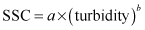
An instream turbidity value, in Formazin Nephelometric Units, associated with each suspended-sediment sample was produced by averaging two or three recorded values over the duration of the sample collection time. An SSC value, in milligrams per liter, was provided by the laboratory analysis of the sample. For all samples collected at a monitoring station, the paired turbidity and SSC data were compiled and transformed to base-10 logarithmic values. These log values were then used to calculate a linear least-squares regression model. The model was converted to the power equation form:
 , (1)
, (1)
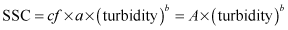
where a and b were the coefficients obtained by the regression analysis. Transformation of the turbidity and SSC data to log values and back to original form introduced a bias into the regression model. The bias was corrected with a “smearing” estimator described by Helsel and Hirsch (1992). The bias correction factor was calculated as the mean of the residual errors from the regression. The final regression model, including the correction factor, had the form:
 , (2)
, (2)
where A was the product of the correction factor (cf) and the coefficient (a) determined by the regression analysis.
The final forms of the regression models for each monitoring station are shown in table 3. The regression models for the seven monitoring stations are plotted in figure 9. For each station, the solid line indicates the estimated SSC that is defined by sample turbidity values used in the regression models. The dashed portion of each line indicates the range of estimated SSC and instream turbidity values at which no suspended-sediment samples were collected.
The regression models for North Santiam, Breitenbush, and Blowout differ from those used to calculate SSC for water years 1999 and 2000 in the previous report by Uhrich and Bragg (2003). Many additional samples were collected at these stations, including some with instream turbidity values greater than 100 FNU. Changes in the USGS rounding protocol for turbidity data also necessitated the exclusion of many samples with low turbidity values (less than 1 FNU) that had been included in the previous models. The removal of these samples from the analyses at North Santiam, Breitenbush, and Blowout resulted in slightly lower R2 values for the regression models at all three stations. However, the inclusion of more high-turbidity samples in the analyses improved the models for estimating SSC from high instream turbidity, when most sediment is transported.
Daily and annual suspended-sediment loads were calculated from the continuous turbidity and streamflow records. The regression model for each monitoring station was used to estimate suspended-sediment concentration from each semi-hourly turbidity value. The semi-hourly suspended-sediment discharge (SSQ) was calculated from the estimated SSC and the instantaneous streamflow (Q) using the following equation:
 , (3)
, (3)
where c = 0.0000562, converting the units to tons per 30 minutes. The 48 semi-hourly SSQ values calculated per day were summed to estimate the daily SSL, in tons. The 365 (or 366) daily SSL values per year were then summed to provide the annual SSL for each station for each water year.
Streamflow data from several gaging stations in the North Santiam River basin were analyzed to provide historical context for the annual mean and maximum instantaneous streamflow for water years 1999–2004 (U.S. Geological Survey, 2000–2005). Five of the water-quality stations were installed at long-term USGS streamflow-gaging stations (North Santiam, Breitenbush, Niagara, Little North, and Mehama; fig. 1). The gaging stations at North Santiam and Breitenbush are located in the upper basin (upstream of Detroit Lake) where streamflow is not affected by operation of the two dams. Niagara and Mehama are both on the mainstem North Santiam River downstream of the dams. Mehama is located nearly 20 mi downstream of Big Cliff Dam with many tributaries (including that gaged at Little North) contributing to the streamflow. Niagara is located less than 1 mi downstream of Big Cliff Dam where streamflow is highly regulated and not responsive to natural flow conditions. Niagara therefore was not included in the historical streamflow analysis.
The streamflow extremes took place during the first 3 years of the 6-year period of study. Annual mean streamflows were highest during water year 1999, when flows at North Santiam, Breitenbush, and Mehama were greater than the 75th percentile (fig. 10). However, the storm producing the peak streamflows occurred in water year 2000. In November 1999, peak flows were greater than the 75th percentile at North Santiam, Breitenbush, and Mehama for their respective periods of record and the peak flow at Little North was greater than the 95th percentile (fig. 11). Streamflows were lowest during water year 2001, when the region experienced a severe drought. The 2001 annual mean streamflows for North Santiam, Breitenbush, Little North, and Mehama were less than the 5th percentile (fig. 10). The peak flows for all four stations also were less than the 5th percentile (fig. 11).
Annual mean and peak streamflows during water years 2002–04 were less extreme than those during water years 1999–2001. Mean annual and peak streamflows generally fell between the 25th and 75th percentiles for all stations during water years 2002-04.

![]() U.S. Department of the Interior | U.S. Geological Survey
U.S. Department of the Interior | U.S. Geological Survey
URL: https://pubs.usgs.gov/sir/2007/5187
Page Contact Information: Publications Team
Page Last Modified: Thursday, 01-Dec-2016 19:51:07 EST
