Scientific Investigations Report 2008-5070
U.S. GEOLOGICAL SURVEY
Scientific Investigations Report 2008-5070
The Stream Network Temperature model (SNTEMP) is a mechanistic, one-dimensional heat transport model that simulates the daily mean and maximum water temperatures as a function of stream distance and environmental heat flux. The model was developed in the early 1980s for the U.S. Department of Agriculture, Soil Conservation Service (Theurer and others, 1984) and has since been used in studies to analyze the effects of reservoir discharge timing, release temperature, and release volume (or some combination of all three) on downstream water temperatures (Bartholow, 2000). The DOS-based SNTEMP (Version 2.0) was used to develop the water-temperature model for this study. The USGS supports and distributes SNTEMP and offers an online course on how to use the model at http://www.fort.usgs.gov/Products/Training/IF312.asp. The SNTEMP software used for this study was obtained online from the USGS Fort Collins Science Center at http://www.fort.usgs.gov/Products/Software/SNTEMP/. The user’s manual (Theurer and others, 1984) contains equations used by the model and describes how to construct model input files. In addition, answers to frequently asked questions about SNTEMP are provided at URL http://www.fort.usgs.gov/products/Publications/4037/4037.asp
The SNTEMP model is composed of the six modules listed in table 2. This table also includes a description of the functionality associated with each module.
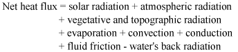
The heat flux module forms the core of the SNTEMP model (Theurer and others, 1984). Processes that affect the amount of heat entering or leaving a stream are represented by the following equation:
 (1)
(1)
The processes represented by the heat flux equation are shown in figure 2. (Energy fluxes directed at the water body are positive and those directed away from the water body are negative.)
The SNTEMP model has several advantages. These advantages include (1) the capability to simulate stream networks of any size or order, and (2) the capability to use a simulation time step ranging from 1 month to 1 day. SNTEMP documentation states that the model is capable of simulating mean water temperatures to within 0.5°C of measured mean water temperatures given representational data for a user selected time step. The model also uses readily available input data and is well documented (Bartholow, 2000).
HDR Engineering, Inc., as part of a study for the State of Idaho Department of Environmental Quality compared several water-temperature models (SNTEMP, Heat Source, Basin Temp, CE-QUAL-W2, CE-QUAL-RIV1, RMA-11, MIKE-11, and hybrid model combinations) and selected SNTEMP to simulate water temperature in the Lochsa River in north-central Idaho based on the criteria that the model should (1) simulate daily maximum stream temperature, (2) be peer-reviewed and used within the scientific community, (3) not require an inordinate amount of time for data collection, and (4) have documentation that is easy to follow and reasonably available technical support (HDR Engineering Inc., 2002).
The SNTEMP model also has limitations. SNTEMP uses a regression equation to estimate daily maximum air temperature, which is used to calculate daily maximum water temperature. The effect of regression equation error on simulation results is discussed in section, “Limitations of Water-Temperature Model”. Technical staff is no longer available as of February 2006 to answer users’ questions about the theory and application of the model. One important fact is that the SNTEMP model does not simulate hydrology flow data and initial water temperatures are required for all input locations.
Five SNTEMP modeled reaches were linked in a series (fig. 3) to simulate daily maximum water temperatures at any given location on the Roza–Prosser Reach, which was required for generating input data for the EDT analytical model.
The equations used in SNTEMP required the length of the modeled reach to approximately equal the distance that a “parcel” of water travels in the reach for the selected simulation time step. For example, if the selected time step is 1 week, then the length of the reach being modeled would be the distance that water would travel in 1 week; if the selected time step is 1 day, then the length of the reach would be the distance that the water would travel in 1 day. The travel time for the Roza–Prosser Reach was determined to be 5 days using water velocity measurements collected by the USGS during field trips in September 2005; therefore, five modeled reaches were necessary to run the model using a daily time step. Because the SNTEMP model is not designed to be linked in series, the USGS linked the modeled reaches by developing software to transform output data from an upstream modeled reach into input for the next downstream modeled reach. The end points for the modeled reaches are shown in figure 3.
The model developed for this study did not use the branch configuration (fig. 4) typical for most stream networks because water temperatures were not simulated for tributaries entering the Roza–Prosser Reach. Instead, the Roza–Prosser Reach was represented as a single channel. Streams, drains, and wasteways carrying water to the Roza–Prosser Reach were designated as point sources; whereas, canals carrying water from the Roza–Prosser Reach were designated as diversions. The water-temperature model requires input of water temperature and flow data for every point source and diversion for every day of the entire simulation period. The structure of the model for the Roza–Prosser Reach with all point sources and diversions is shown in figure 5. The vertical line in figure 5 represents the Roza–Prosser Reach. Entities listed left of the vertical line are adding water to the Roza–Prosser Reach; whereas, sites listed to the right of the vertical line are entities diverting water from the Roza–Prosser Reach.
Simulated daily maximum water temperature from SNTEMP was generated for locations that correspond to the input locations for the EDT analytical model (fig. 6). An example of the output file generated for input into the EDT analytical model is shown in appendix A.
SNTEMP model was designed to use data that are relatively easy to gather from maps and Federal data sources (Bartholow, 2000). Because SNTEMP is a steady-state model and uses a daily time step, the model requires daily mean data as input.
SNTEMP model requires daily mean values for air temperature, relative humidity, wind speed, and solar radiation or percent cloud cover for each day of the simulation period. Precipitation data are not used because the model does not simulate flows. The AgriMet weather station in Harrah, Washington (fig. 7) was used to obtain values for mean air temperature, relative humidity, wind speed, and solar radiation, which were used for calibration and testing simulations. The weather data were downloaded from the web site http://www.usbr.gov/pn/agrimet/webarcread.html for the station code HRHW. Data for these four meteorology parameters from January 1, 1988, through October 31, 2006, are shown in figure 8. The boxplots illustrate general weather patterns for the Roza–Prosser Reach; namely, relative humidity is inversely related to air temperature and solar radiation. The boxplot for wind speed shows that wind speed is fairly constant throughout the simulation period.
Solar radiation, daily mean air temperature, and daily mean relative humidity data from July 4 through September 30, 2006, were collected at four USGS weather stations at Roza, Parker, Granger, and Prosser, Washington. (fig. 7). These weather data were compared to weather data from the AgriMet weather station (Harrah, Washington) to determine whether data from the AgriMet station represented conditions near the river. If the data did not represent these conditions, then appropriate adjustments to the data were needed before the data were used as input to the model. Scatter plots showing these comparisons are shown in figure 9. Correlation coefficients for the weather data from the AgriMet weather station at Harrah, Washington, and data from the four USGS weather stations were 0.97 or greater for daily mean air temperature (fig. 9A), 0.94 or greater for solar radiation (fig. 9B), and 0.83 or greater for relative humidity (fig. 9C). The high correlations provide evidence that the weather data from the AgriMet weather station at Harrah, Washington, is representative of weather conditions along the Roza–Prosser Reach, and adjustments were not made to the AgriMet weather data before using the data for model input.
SNTEMP model does not simulate hydrology. Therefore, before the model could be run, flow data needed to be determined at all locations where flow enters or leaves the Roza–Prosser Reach for each time step during the simulation period. Flow data were obtained from two sources: Hydromet gaging stations maintained by the Bureau of Reclamation and field measurements collected in September 2005 by the USGS.
Average daily flow data for model calibration and testing were downloaded for 15 gages from the Bureau of Reclamation’s Yakima Project Hydromet System Web page at http://www.usbr.gov/pn/hydromet/yakima/index.html. The Hydromet system is a network of automated hydrologic and meteorological monitoring stations located throughout the Pacific Northwest. Remote data collection platforms transmit water and environmental data by using point-to-point radio or satellite communications to provide near-real-time water management capability. The sites used to supply data to the model are listed in table 3.
From September 14 through September 16, 2005, the USGS measured flows in the Roza–Prosser Reach and at more than 40 joining creeks, diversions, wasteways, and drains, which are referred to as laterals. Sites used to estimate flows for the water-temperature model are listed in table 4, and the locations of the sites are shown in figure 10.
A database table was developed to include columns for flow and water temperature for each of the 15 Hydromet gaging stations and for the laterals sampled by the USGS. Data for the 15 Hydromet gaging stations were then imported into this database table. The flow to and from the Roza–Prosser Reach from ungaged laterals was calculated using the following methods:
There are no diversions for this section of the Roza–Prosser Reach. Inflow from April through September is mostly water used for irrigation returning to the Roza–Prosser Reach through laterals.
There is one gaged diversion for this section of the Roza–Prosser Reach. Inflow from April through September is mostly water used for irrigation returning to the reach through laterals.
Ground water flowing to and from a river affects water temperature (Poole and Berman, 2001) and is an important process, but difficult to measure. The SNTEMP model sets ground-water flow equal to the difference between inflow and outflow. For example, if flow into the model is 20 m3/s and the outflow from the model is 21 m3/s, then the model will add 1 m3/s as ground-water inflow. The model sets the temperature of the ground water equal to the mean annual air temperature for the simulation period, unless the user specifies another value. Ground-water temperature was set to 11.2ºC for calibration and testing simulations based on the calculated average daily mean air temperature at the AgriMet weather station (Harrah) from January 1, 1988, through December 31, 2005. SNTEMP adds ground water to a model as a distributed flow, meaning that flow in a reach was added equally throughout the reach of the entire model instead of being discharged at a specific location.
Water temperature, as with flow, must be determined for all inflows before the SNTEMP model can be run. However, consistent water-temperature data for flows into the Roza–Prosser Reach were not available, and methods needed to be developed for estimating inflow water temperatures. Water temperatures leaving the Roza–Prosser Reach do not need to be calculated because those temperatures do not affect the temperature of the Roza–Prosser Reach, and outflow water temperatures are not used in other calculations. Two methods were developed by the USGS to estimate the water temperature of flows entering the Roza–Prosser Reach: (1) regression equations to estimate water temperatures for rivers entering the Roza–Prosser Reach (namely the upper Yakima River above Roza Diversion Dam and the Naches River where the river joins the Roza–Prosser Reach just north of Yakima) and (2) a set of regression equations to estimate water temperature for all streams, wasteways, and drains entering the length of the Roza–Prosser Reach.
To develop the regression equations for the Yakima River above Roza Diversion Dam and the Naches River where the river joins the Roza–Prosser Reach, existing datasets were required for water temperature (response variable) at both locations as well as for other parameters used to explain the variations in water temperature over time (explanatory variables). Daily records of average water temperature at both locations were obtained from the Bureau of Reclamation Hydromet database (table 5).
The primary dataset used to derive explanatory variables for Roza Diversion Dam and Naches River regressions was obtained from the National Climate Data Center (NCDC). Specifically, the daily mean air temperature recorded at Yakima Air Terminal (Site ID: YKM) was used. Previous studies have concluded that in the absence of other data, mean air temperature (above freezing) can explain most variations in water temperature (Bartholow, 1989). For the Naches River regression, river discharge recorded at the Naches River at Yakima gaging station also was used. Because the model alternatives were seasonal and limited to the 7-month period April 1 through October 31, only data collected during this period were used to develop the regression equations.
Regression equations were derived by using S-PLUS statistical software (Insightful Corp., 2002). Ordinary least-squares (OLS) linear regression as well as linear robust (least trimmed squares, LTS) and nonlinear methods were considered. Initially, a regression equation was developed to estimate water temperature, using only daily mean air temperature as an explanatory variable. Residual plots for these regressions (residual versus fit) showed slight curvature (heteroscadasticity) that resulted in a relation between residuals and the explanatory variable that was not desirable and likely the result of seasonality. To incorporate the effect of seasonality, regressions were examined using 3-, 7-, 15-, 30-, and 45-day moving averages of air temperature and a time-dependent parameter based on a function of Julian day. In the case of the Naches River regression, river flow also was added. Then a stepwise regression technique was used to select variables that best explain the data variance, thereby reducing the total number of variables. An evaluation of multi-colinearity between variables (Helsel and Hirsch, 1995) also was performed and further reduced the number of variables.
The resulting linear regression equations for estimating water temperature at Roza Diversion Dam and Naches River at Yakima are:
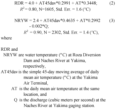
Explanatory variables need not be independent of each other (Helsel and Hirsch, 1995), and although the explanatory variables AT45dav and AT are derivations of the same parameter, these variables are only modestly correlated (r = 0.65).
The proportion of variability (R2) explained by using robust LTS or nonlinear regression methods did not increase appreciably, nor was there a substantial decrease in standard error; therefore these methods were not used.
An important assumption for the regression equation for the Roza Diversion Dam is that water temperature near the surface of the reservoir (at the location of the sensor) is representative of water temperature in the river immediately downstream of the spillway. The water temperature sensor was located just west of the gage structure on the dam, about 46 meters from the edge of the spillway (Q. Kreutler, U.S. Bureau of Reclamation, written commun., 2006). Water temperature data collected by the USGS between April 1 and July 20, 2006, indicated that on average the water temperature at the gaging station was within 0.2ºC of water temperature in the river immediately downstream of the spillway.
Water temperature for inflowing lateral sites was estimated by developing regression equations for 11 inflowing laterals that had limited measured water temperature data available (table 6). Other inflowing laterals to the Roza–Prosser Reach were then assigned the same water temperature as the nearest lateral with a developed regression equation for water temperature (see appendix C).
Stream geometry data were developed to define characteristics of the Roza–Prosser Reach. The SNTEMP model requires descriptive data for the model nodes and the river sections between the nodes. Model nodes are used in the Roza–Prosser Reach to define where model sections begin and end, where water enters or leaves the reach, where simulation results are output, and where substantial changes occur in reach characteristics. Each model node must be assigned a site location (distance upstream for some arbitrary downstream site), latitude, and elevation, which were derived using a Geographic Information System (GIS) in this study. Reaches between points require data for the reach azimuth (defined as the deviation of a channel from a true north-south axis), the river roughness coefficient called Manning’s N, and width of the river. Reach properties are set at the starting node and are considered constant until these properties are changed at a node farther downstream.
A GIS was used to determine the azimuth for sections of the Roza–Prosser Reach. A Manning’s N value of 0.04 (the value for large natural channels) was selected from the SNTEMP user’s manual (Table II, page II-3) and was assigned to all channels in the Roza–Prosser Reach. The width of a river can be set to a constant value or can vary with flow. The equation W = aQb (where W is stream width in meters, Q is flow in cubic meters per second, and a and b are coefficients) was used to change the width of reaches as the flow changed. The equation coefficients a and b were determined by using the results of the Bureau of Reclamation’s HEC-RAS model, which estimates channel width for a set of flow conditions for hundreds of cross sections along the length of the Roza–Prosser Reach. The equations derived from the HEC-RAS model also represent sections of the reach that had braided channels.
Shading lowers water temperature by reducing the amount of solar radiation that enters the water. To test for the effect that shading might have on water temperature in the Roza–Prosser Reach, a shading survey was conducted by the USGS on October 26–28, 2006, at 37 stations, covering a total river distance of 62 km.
The shading survey methods used were developed by previous researchers (Quigley, 1981; Theurer and others, 1984) and outlined more recently by Bartholow (1989). Parameters measured at each station were date, time, location, stream azimuth, stream width, topographic altitude, vegetation shade parameters, and incident solar radiation. Location and stream azimuth were determined using a standard compass and Global Positioning System (GPS). A hand-held LaserAce Hypsometer was used to measure stream width, topographic altitude, and vegetation shade parameters, including height above water surface, crown width, distance from the edge of the water, and vegetation density. Vegetation density is partly subjective and was determined by estimating the percentage of continuity of vegetation (quantity) along the river reach and multiplying this by the percentage of incident solar radiation filtered through the vegetation (quality).
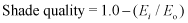
Incident solar radiation measurements were made by using a hand-held solarimeter. Direct solar radiation was measured from the center of the river, exposure measurement in sunlight (Eo), and diffuse solar radiation was measured at the riverbank, exposure measurement in shade (Ei). Bartholow (1989) used both incident solar radiation measurements to determine a relative shade quality index:
In addition to the above measurements, digital photographs were taken at each station, and the water temperature was measured.
Two hydrographers collected measurements from a 5-m jet boat with a 35-horsepower outboard motor. The river generally was navigable at the time of the survey, and the boat was used to travel between stations, allowing observation of various riparian terrain and vegetation.
Weather conditions at the time of the survey were mild, dry, and generally clear. The level of sunlight was not constant during the survey and changed frequently during the days because of intermittent clouds. Following the suggestion of Bartholow (1989), shade data mostly were collected between 0900 and 1500 hours. The locations where shade measurements were collected are shown in figure 11, and an example of the field sheet is in appendix D.
For this project, shading data were entered into the model for locations where shade was directly measured. Estimates of shading at other locations were based on relating shading measurements to orthophotographs. Sections of the Roza–Prosser Reach that appeared similar to measured sections were given average values of the measured sections.
Topographic shading was not estimated in the field by the USGS because topographic shading is difficult to measure and is usually not a factor for large rivers in a floodplain. However, the upper regions of the study area are in a canyon where topographic shading may contribute to a decrease in water temperature. In the future, topographic shading in the canyon could potentially be calculated using a GIS and digital elevation data, but this calculation was beyond the scope of this study.

![]() U.S. Department of the Interior | U.S. Geological Survey
U.S. Department of the Interior | U.S. Geological Survey
URL: http://pubs.usgs.gov/sir/2008/5070
Page Contact Information: Publications Team
Page Last Modified: Thursday, 10-Jan-2013 18:47:09 EST
