USGS Home
Contact USGS
Search USGS

U.S. GEOLOGICAL SURVEY
Scientific Investigations Report 2008–5201

Back to Table of Contents

Methods

Continuous Water Quality Monitors

YSI model 600XLM or model 6920 continuous water quality monitors (“sondes”) were placed at 2 sites in Agency Lake and 17 sites in Upper Klamath Lake (fig. 2, table 1). In Upper Klamath Lake, 12 monitors were in open-water areas and 5 monitors were in nearshore areas (5–10 m from shore or in reed beds adjacent to the open lake). Nearshore sites were HPK, SHL, SSR, GBE, and WDW. Water quality monitoring locations in open-water areas of Upper Klamath Lake were similar to those in 2005 (fig. 3), but with some changes based on an evolving understanding of the lake system that were made to optimize the data collection effort. For example, several years of monitoring conditions in Shoalwater, Ball, and Howard Bays has established that the bays are largely disconnected from the rest of the lake in terms of the seasonal dynamics of water quality. Although the data are interesting because they quantify extremes in water quality conditions, they add little to the objective of understanding the water quality dynamics in the open-waters of the lake. For this reason, two bay sites (BLB and SHB, fig. 3) were discontinued and two sites were added at the northern and southern extremes of the deep trench on the western side of the lake (sites EBB and SET, fig. 2). In addition, the sites MPT and MDL were determined to be redundant and were replaced by the single site MRM. Meteorological data collection continued at the MDL site.

At most continuous water quality monitoring locations, sondes were placed vertically at a fixed depth of 1 m from the lake bottom; if the depth at a site was less than 2 m, the sonde was placed horizontally at the midpoint of the water column. A typical sonde mooring is shown in figure 4. Placing the sonde 1 m from lake bottom provided data relevant to the endangered botton-feeding suckers of Upper Klamath Lake. To monitor water quality conditions near the water surface and provide comparisons to conditions near the lake bottom, a second sonde was placed on the same mooring at a fixed depth 1 m from the surface at the four deepest sites, SET, MDT, EPT, and MDN (fig. 2). All sondes recorded sonde depth, dissolved oxygen concentration, pH, specific conductance, and temperature at the beginning of every hour.

Sondes were cleaned and field measurements of site depth were made during weekly site visits to ensure proper placement of the instrument in the water column. Separate field measurements of dissolved oxygen concentration, pH, specific conductance, and temperature at the depth of the site sonde were made as an additional check of sonde performance. Deployments generally lasted 3 weeks, and then the sonde at the site was replaced with a newly calibrated instrument. Calibration of each parameter was checked in the laboratory after sonde retrieval to measure calibration drift. The raw data were then uploaded to the USGS automated data processing system (ADAPS). Quality of the data was assured by the field information collected at weekly site visits and by processing the time series according to the procedures in Wagner and others (2006). Corrections to data due to biological fouling and drift as determined during the post-deployment calibration check were entered into ADAPS, which calculated the corrected values.

Water Sample Collection

Water samples were collected on a weekly basis according to established protocols (U.S. Geological Survey, variously dated). Samples were analyzed for chlorophyll a, total phosphorus, total nitrogen, ammonia (includes ammonia plus ammonium), orthophosphate, and nitrite-plus-nitrate concentrations. A subset of the continuous water quality monitoring sites, MDN, WMR, EPT, MDT, HDB, and RPT (fig. 2), were selected for the sampling. Two methods of sampling were used. The choice of method depended on the category of analyte to be measured. Water samples analyzed for total phosphorus, total nitrogen, and chlorophyll a were collected using methods designed to achieve an equal integration over the depth of the water column. To collect depth-integrated samples, a weighted cage holding two 1-L bottles was lowered at a constant rate into the water to 0.5 m from the bottom at sites less than 10.5 m depth (“shallow” sites) and to 10 m from the surface at sites greater than 10.5 m depth (“deep” sites). Each bottle had two ports, one for water to flow in, and one for the escape of displaced air. The contents of bottles from multiple collections at a site were composited, mixed, and then split into separate fractions using a churn splitter.

At the beginning of the sampling season in May, water samples analyzed for dissolved nutrients (ammonia, orthophosphate, and nitrite-plus-nitrate) were collected from a point mid-depth in the water column at sites MDN, WMR, HDB, and RPT, and at two points in the water column (at one-quarter and three-quarters of the total depth) at sites MDT and EPT. Point samples were collected by lowering one end of a hose to the appropriate depth in the water column, then passing the sample through a 0.45 µm capsule filter using a peristaltic pump. After July 1, sites MDN, WMR, and HDB were discontinued to meet logistical and resource constraints. The sampling protocol at RPT, MDT, and EPT was changed to collection of a sample just below the water surface and another sample 5 m below the water surface (RPT sample was just below water surface only), to support the objectives of a parallel study of AFA buoyancy by Portland State University (J. Rueter, Portland State University, oral commun., 2006).

Dissolved nutrient, total phosphorus, and total nitrogen samples were chilled on site and sent to the National Water Quality Laboratory (NWQL) in Denver, Colorado, for analysis. Total phosphorus and total nitrogen samples were preserved in the field with 1 mL of 4.5 normal (4.5N) H₂S0₄ (Sulfuric Acid). Finalized data were stored in the USGS National Water Information System (NWIS) database. Samples for chlorophyll a concentrations were passed through a 0.45 µm glass fiber filter, and the filter membrane was frozen and sent to Portland State University in Portland, Oregon, for analysis. Because samples were processed at Portland State University, the results of the chlorophyll a analyses were not stored in the USGS NWIS database. The comparability of Portland State University and NWQL chlorophyll a data was established with four interlaboratory splits, two of which were submitted to two laboratories in addition to Portland State University and NWQL. Chlorophyll a samples were analyzed according to Arar and Collins (1997).

To protect samples from contamination during the collection process, quality control protocols were followed as described in the National Field Manual for the Collection of Water-Quality Data (U.S. Geological Survey, variously dated). Although all quality assurance protocols were followed to ensure accuracy, there was evidence of minor contamination in ammonia and total nitrogen blank samples; the results are discussed further in appendix A. Less than one-half of blank samples were contaminated, and the magnitude of seasonal differences in environmental samples was greater than the error associated with potential contamination.

Dissolved Oxygen Production and Consumption Experiments

Between mid-June and mid-October, experiments were conducted to obtain direct measurements of gross dissolved oxygen production and consumption rates at six sites—MDN, WMR, RPT, HDB, MDT, and EPT—in Upper Klamath Lake (fig. 5). Biological oxygen demand (BOD) bottles, with a volume of 300 mL and made of type 1 borosilicate glass, were filled with lake water integrated from the entire water column. BOD bottles were filled from the churn splitter with the same collection of lake water as for chlorophyll a samples. This procedure allowed the chlorophyll a data to be used in the analysis of data from the dissolved oxygen production and consumption experiments. Immediately after filling the bottles, initial dissolved oxygen concentration and temperature were measured by using a YSI model 52 dissolved oxygen meter. Three bottles were attached to rest horizontally on racks at each of two depths. One bottle in each group of three was dark (made so by wrapping the bottle and stopper with black electrical tape). Once attached to the incubator rack, the bottles were lowered into the water.

The experimental apparatus was moored at the site for at least 45 minutes and typically retrieved before 3 hours had elapsed. Dissolved oxygen concentration and temperature were again measured in each bottle, and incubation time was noted. The change in dissolved oxygen was calculated in each bottle, and the incubation time was used to express the rate of dissolved oxygen change in milligrams per liter per hour [(mg/L)/h]. The upper and lower racks were positioned 0.5 and 1.5 m below water surface, respectively. Toward the end of the season, as the lake level declined, the lower rack was raised to 1 m depth at the shallow sites (table 2). Some sites were too shallow toward the end of the field season to incorporate the lower rack into the experiment.

Light intensity was measured in a vertical profile from the water surface to 2.5 m depth (or the lake bottom) in 0.5 m increments by using a LiCor LI-193SB underwater spherical quantum sensor. These measurements were used to estimate the depth of the photic zone, defined here as the point at which 99 percent of incident light is absorbed (or, 1 percent of incident light is transmitted), by using Beer’s law, which describes the penetration of solar radiation through the water column as an exponential relation:

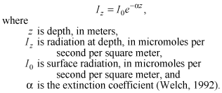(1)

At each set of measurements, α was estimated by fitting equation (1) to the vertical profile of the light meter readings. The depth of the photic zone () was then calculated as

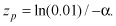(2)

Measurements of the vertical profile of light intensity were made at each site on each date at the beginning (“early” measurements) and immediately after the incubation period (“late” measurements). These two profiles were combined to provide the average depth of photic zone throughout the duration of each experiment at each site.

An estimate of the potential change in dissolved oxygen over a 24-hour period (∆DO) was made from the measured oxygen production and consumption rates in the light and dark bottles. The gross production, G, in (mg/L)/h was assumed to have the same exponential dependence with depth as light radiation. Then, in analogy with equation 1, the gross production at any depth in the water column G_z as a function of the gross production at the water surface G₀ is given by

(3)

The above equation can be solved for G₀ in terms of the value obtained from the rack at 0.5 m depth

(4)

The gross production integrated over a water column of depth D, denoted G, is given by

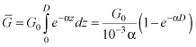(5)

where 10^-3 is a proportionality constant and the units of G are (mg/m²)/h.

Respiration rates (R) were similar in both racks, and were assumed constant throughout the water column for this calculation. Respiration integrated over the water column is given by

(6)

where 10^-3 is a proportionality constant. The units of R are (mg/m²)/h. The final simplification is to assume that the gross production rate is constant at G for 12 hours of daylight in every 24 hours and zero for the remaining 12 hours, and that the respiration rate is constant for a full 24 hours. Then the estimated change in dissolved oxygen over a 24-hour period, expressed in terms of a concentration (mg/L), is

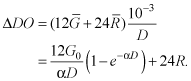(7)

Meteorological Sites

The locations of meteorological measurement sites in Upper Klamath Lake are shown in figure 2 and listed in table 3. All meteorological sites were in the same locations as the study in 2005.

A diagram of the typical land-based meteorological site is shown in figure 6. Wind speed and direction data were collected by an RM Young model 05103 wind monitor. Air temperature and relative humidity data were collected by a Campbell Scientific CS500 or HMP35C relative humidity and air temperature sensor. Additionally, solar radiation data were collected at the WMR MET site using a Li-Cor LI200SZ pyranometer and at the SSHR MET site using an Eppley model PSP pyranometer. Floating sites were similar to the land-based sites, although the mast attached to the buoy provided a height, measured from the surface of the water, of 2 m for wind monitors and 1.5 m for relative humidity and temperature sensors. Relative humidity and temperature data were not collected at the MDN MET site during the 2006 field season. Data collected from all sensors at a site were stored every 10 minutes by a Campbell Scientific CR510, CR10, or CR10X datalogger at the station. A 12-volt battery at the station charged by a solar power array provided power. Data were collected during site visits approximately every 2 weeks during the field season. During these visits, sensors were checked for proper function by comparison with hand-held instruments and were cleaned and maintained as needed. Information necessary to correct data due to drifts from proper calibration was collected as needed. Raw meteorological data also were loaded into ADAPS and processed in the same manner as the water quality monitor data.

Data Processing

Before calculating statistics, data from continuous water quality monitors were screened using temporal and, when appropriate for the statistic, spatial criteria. For this report, daily statistics were used for continuous water quality monitor data. To ensure that data were acceptable to compute daily statistics, at least 80 percent of measurements from one site for one day had to be present, which would constitute a “qualifying day” of data. A spatial criterion was applied when data collected from the entire lake were compiled to compute a statistic, such as lakewide daily median dissolved oxygen. This criterion specified that at least 70 percent of water quality sites in the lake had to have qualifying daily data to compute the lakewide statistic for a particular day.

For statistics at individual meteorological sites, the temporal criterion ensured that at least 80 percent of possible measurements made in one day were present to constitute a qualifying day of data. To compute lakewide meteorological statistics, different levels of spatial acceptability were applied depending on the parameter because not all parameters were collected at all sites, and relatively few meteorological stations were installed around the Upper Klamath Lake basin. Air temperature and relative humidity measurements were collected at five sites, so the spatial criterion for these parameters ensured that daily qualifying data were available at four of the five sites (80 percent) to compute a lakewide daily statistic. Wind speed data were collected at all meteorological sites, so the spatial criterion for wind speed ensured that five of the six sites (83 percent) had daily qualifying data to compute a lakewide daily statistic. Because solar radiation data were collected at only two sites, these data were not screened according to spatial criteria.

Back to Table of Contents