Techniques and Methods 6-A19
U.S. GEOLOGICAL SURVEY
Techniques and Methods 6-A19
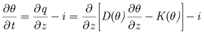
Vertical flow through a homogeneous unsaturated zone can be approximated with kinematic waves (Colbeck, 1972; Smith, 1983; Smith and Hebbert, 1983; Charbeneau, 1984). This approximation is made by simplifying Richards’ equation, which can be written in the vertical dimension as:
 ,
(1)
,
(1)
where
is |
the volumetric water content (volume of water per volume of rock); |
|
is |
the water flux (volume of water per time per unit area); |
|
is |
the elevation in the vertical direction (length); |
|
is |
the hydraulic diffusivity (length squared per time); |
|
is |
the unsaturated hydraulic conductivity as a function of water content (length per time); |
|
is |
the ET rate per unit depth (length per time per length); and |
|
is |
time. |
If equation 1 is simplified to remove the diffusive term, assuming that the vertical flux is only driven by gravitational forces, the vertical flux owing to gravity is:
 ,
(2)
,
(2)
where
is |
shown as negative downward. |
Substituting equation 2 into equation 1, neglecting![]()
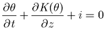
(the diffusive term), and assuming evaporation is removed from the soil profile instantaneously and all flow is downward vertical yields:
 .
(3)
.
(3)
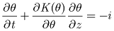
The method of characteristics solution to equation
3 is obtained by rewriting equation 3 so that ![]() is taken partially in terms of
is taken partially in terms of ![]() and
and ![]() :
:
 ,
(4)
,
(4)
and by introducing the equation of variation (Abbott, 1966):
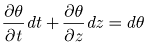 .
(5)
.
(5)
Equations 4 and 5 written in matrix form yields:
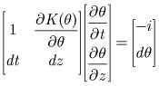 .
(6)
.
(6)
![]() and
and ![]() must be indeterminate along characteristic lines (Abbott, 1966). This occurs
only when the determinant of the coefficient matrix in equation 6 and the determinants
of the matrices obtained by substituting the right hand side vector for each
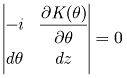
column in the coefficient matrix are all zero, as described in equation 7:
must be indeterminate along characteristic lines (Abbott, 1966). This occurs
only when the determinant of the coefficient matrix in equation 6 and the determinants
of the matrices obtained by substituting the right hand side vector for each
column in the coefficient matrix are all zero, as described in equation 7:
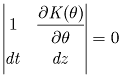 ,
(7a)
,
(7a)
 ,
(7b)
,
(7b)
 .
(7c)
.
(7c)
Expanding the determinants yields:
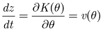 ,
(8a)
,
(8a)
 ,
(8b)
,
(8b)
 ,
(8c)
,
(8c)
where
is |
the characteristic velocity restricted to the downward
(positive |
The characteristic equations 8a, b, and c define the velocity of a wave, the change in water content of the wave with time, and the change in water content with depth behind the wave, respectively. This wave represents a wetting front in the unsaturated zone that was generated by a sudden increase in infiltration at land surface and that is being affected by ET. Without ET, the water content of the wave is constant over the wave profile. However, the inclusion of ET creates a
non-linear slope ![]() in water content over the wave profile
in water content over the wave profile
if a non-linear function for ![]() is used, such as the Brooks‑Corey function (Brooks and Corey, 1966).
is used, such as the Brooks‑Corey function (Brooks and Corey, 1966).
The derivative ![]() is discontinuous over a sharp
is discontinuous over a sharp
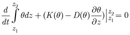
wetting front that results from neglecting the diffusive term in equation 1, such that the spatial derivative in equation 3 is not defined in the absence of hydraulic diffusion. An analytic solution for the velocity may still be derived by considering the effects of diffusion and substituting an equivalent sharp wetting front of equal mass (Smith, 1983; Charbeneau, 1984). The solution to equation 1 for a wetting front that considers hydraulic diffusion can be found by integrating over a control volume containing a single wetting front (Charbeneau, 1984):
 ,
(9)
,
(9)
where
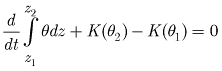
and distances far enough that |
![]() can be neglected because
can be neglected because ![]() at
at ![]() and
and ![]() such that:
such that:
 ,
(10)
,
(10)
where
and |
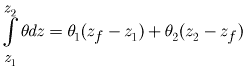
Integrating over a profile containing a sharp front with equivalent mass gives:
 ,
(11)
,
(11)
where
is |
the depth of the sharp front. |
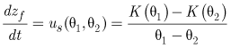
Combining equations 10 and 11 gives:
 ,
(12)
,
(12)
where
is |
the velocity of a sharp wetting front (length per time); |
|
is |
the volumetric water content above a depth |
|
is |
the volumetric water content below a depth |
An increase in the infiltration rate will cause a wetting front to form, which is represented by a lead wave. A decrease in the infiltration rate will cause a drying front to occur, which is represented by a trailing wave. Thus, waves are used to represent both wetting and drying fronts. Attenuation of a lead wave occurs as a trailing wave of higher velocity overtakes it. When a trailing wave overtakes a lead wave, the water content of the lead wave becomes equal to the water content of the trailing wave. Consequently, this reduces the velocity of the lead wave. Conversely, when a lead wave overtakes a trailing wave or another lead wave of lower velocity, the overtaken wave is removed, and the water content and flux of the uppermost lead wave are maintained, resulting in rewetting. The process of waves intercepting each other is termed a shock, and this process is important to the method of characteristics because wave properties, such as water content and flux, become discontinuous at the instant a shock occurs (Abbott, 1966).
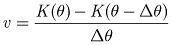
In contrast to a wetting front that stays sharp, trailing waves elongate with time owing to gravity. Consequently, trailing waves must be divided into a series of incremental waves or be represented by a function that describes internal drainage with time. In either case, internal drainage is determined based on the water content and relative location of points along a trailing wave. For example, points A and B shown in figure 2 represent two points along the trailing wave where the velocities may be determined. The velocity at points A and B is calculated from the characteristic solution (equation 8a) and the ratio of their velocities is equal to the ratio of their depths:
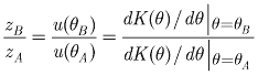 ,
(13)
,
(13)
where
is |
the depth of the trailing wave increment below land surface represented by point A in figure 2, and |
|
is |
the depth of trailing wave increment below land surface represented by point B in figure 2. |
In contrast to a lead wave that forms a discontinuity
in the water content profile, the derivative ![]() is continuous over a trailing front. Accordingly, the Brooks-Corey unsaturated
hydraulic conductivity function can be used to evaluate
is continuous over a trailing front. Accordingly, the Brooks-Corey unsaturated
hydraulic conductivity function can be used to evaluate ![]() .
The Brooks-Corey function for unsaturated hydraulic conductivity can be expressed
as:
.
The Brooks-Corey function for unsaturated hydraulic conductivity can be expressed
as:
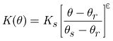 ,
(14)
,
(14)
where
is |
the saturated hydraulic conductivity; |
|
is |
the residual water content; |
|
is |
the saturated water content; and |
|
is |
the Brooks-Corey exponent. |
The drainable water from an unconfined or water-table
aquifer, referred to as the specific yield or ![]() ,
is equal to the porosity minus the specific retention
,
is equal to the porosity minus the specific retention ![]() ,
where
,
where ![]() is the volume of water per unit volume of rock that is retained when the rock
is drained by gravity (Meinzer, 1923, p. 28). Specific yield is used by MODFLOW-2005
to calculate the amount of storage within an unconfined aquifer. Thus, continuity
between the unsaturated zone and unconfined aquifers in MODFLOW-2005 is maintained
through the specific yield by approximating
is the volume of water per unit volume of rock that is retained when the rock
is drained by gravity (Meinzer, 1923, p. 28). Specific yield is used by MODFLOW-2005
to calculate the amount of storage within an unconfined aquifer. Thus, continuity
between the unsaturated zone and unconfined aquifers in MODFLOW-2005 is maintained
through the specific yield by approximating ![]() .
Residual water content generally is smaller than
.
Residual water content generally is smaller than ![]() ,
such that caution should be used when representing unsaturated flow parameters
in the UZF1 Package with measured values.
,
such that caution should be used when representing unsaturated flow parameters
in the UZF1 Package with measured values.
The velocity of the deepest point along a trailing
wave is determined by taking the derivative of equation 14 with respect to ![]() :
:
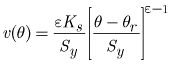 ,
(15)
,
(15)
where
and |
A relation between the deepest point along a trailing wave and all other points along a trailing wave is determined by substituting the velocity defined by equation 15 into equation 13 and results in:
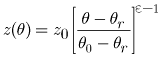 ,
(16)
,
(16)
where
is |
the depth of a point on a trailing wave; |
|
is |
the water content of a point on a trailing wave; and |
|
and |
||
For example, the depths of points along a trailing wave may be generated
by choosing water content values between ![]() and
and ![]() shown in figure 2 and by using equation 16 to calculate
the depth at a particular time following a decrease in the infiltration rate.
Thus, equation 15 may be used to calculate the velocity and the corresponding
depth of the front of a trailing wave and then equation 16 can be used to determine
the drainage profile above the trailing front.
shown in figure 2 and by using equation 16 to calculate
the depth at a particular time following a decrease in the infiltration rate.
Thus, equation 15 may be used to calculate the velocity and the corresponding
depth of the front of a trailing wave and then equation 16 can be used to determine
the drainage profile above the trailing front.
During a pulse of infiltration, a lead wave’s velocity and water content will decay during a subsequent period of less infiltration as trailing waves overcome the lead wave. The spreading of a trailing wave caused by gravity is defined by equations 15 and 16; however, these equations are not applicable after a trailing wave has intercepted a lead wave. Analytic relations can be derived for routing trailing waves during interception with a lead wave but these equations are difficult to solve. A simpler approach is to divide the trailing wave into steps or increments and calculate velocities of each increment based on a finite-difference approximation (Smith, 1983):
 ,
(17)
,
(17)
where
is |
the change in water content between two adjacent locations along a trailing wave. |
The UZF1 Package relies on equations 15 and 16 to route trailing waves until the trailing waves intercept another lead wave, at which point the trailing wave is discretized into multiple waves that are routed according to equation 17.
The finite-difference approximation of the true trailing wave as depicted in figure 2 does not conserve mass perfectly when a trailing wave intercepts a lead wave and vice versa. However, for problems involving rapidly varying infiltration rates, mass is conserved within an error of less than 0.05 percent when each trailing wave is represented by 15 increments, although 10 increments are sufficient for most problems to achieve a mass balance error of less than 0.05 percent. The user specifies the number of increments used to represent a trailing wave with the UZF1 Package input parameter NSTRAIL.
As described, waves are generated by changes in the
infiltration rate and will have differing velocities leading to the possibility
of shocks. Determination of the timing of shocks is required for modeling because
the wave properties (![]() ,
,
![]() )
become discontinuous in time and have to be recalculated in order to continue
the solution. Thus, the UZF1 Package routinely calculates the shortest time
for any two waves to intersect. Waves are routed continuously between wave intersections,
while wave properties remain constant. Consequently, the UZF1 Package requires
a unique time discretization that is specific to the problem being solved; the
UZF1 Package time steps are different than those used in MODFLOW-2005.
)
become discontinuous in time and have to be recalculated in order to continue
the solution. Thus, the UZF1 Package routinely calculates the shortest time
for any two waves to intersect. Waves are routed continuously between wave intersections,
while wave properties remain constant. Consequently, the UZF1 Package requires
a unique time discretization that is specific to the problem being solved; the
UZF1 Package time steps are different than those used in MODFLOW-2005.
Evaporation and uptake by roots in the unsaturated zone can cause negative potential gradients, such that diffusive forces can be important. Evaporation can cause water to move upward in the unsaturated zone by drying out the soil at land surface. These conditions cannot be modeled with kinematic waves because diffusive forces are neglected. However, infiltrating water affected by evaporation and uptake by roots can be approximated with kinematic waves during relatively wet conditions because negative potential gradients are less important. This approach assumes that evaporation and uptake by roots can be grouped together as ET, and that they occur as an instantaneous loss of water over a depth interval equal to the depth of root uptake.
Assuming that ![]() is independent of
is independent of ![]() ,
equations 8b and 8c can be integrated to find:
,
equations 8b and 8c can be integrated to find:
 ,
(18a)
,
(18a)
 ,
(18b)
,
(18b)
where
is |
the water content at the head of a lead wave above the
ET extinction depth after time |
|
is |
the water content at the head of a lead wave after time
|
ET is specified as a rate (length per time) within the UZF1 Package (input variable PET) and is converted internally to a rate per unit depth by dividing the specified ET rate by the extinction depth (EXTDP).
Equation 18a is used to calculate the water content
at the head of a lead wave through time and equation 18b is used to calculate
the depth of points along the leading-wave profile between ![]() and
and ![]() ,
where
,
where ![]() is the water content at land surface corresponding to the infiltration rate
is the water content at land surface corresponding to the infiltration rate
![]() , and
, and ![]() and
and![]() are the water contents at arbitrary points along the lead-wave profile with
are the water contents at arbitrary points along the lead-wave profile with
![]() being deeper than
being deeper than ![]() (fig. 3). The water content of a trailing wave is
decreased according to the ET rate and equation 18a. If the water table elevation
is above the extinction depth and the ET demand is not met by the unsaturated
zone, then ET is removed directly from ground water. ET is removed from ground
water using the same method implemented in the MODFLOW ET Package (McDonald
and Harbaugh, 1988, p. 10-1).
(fig. 3). The water content of a trailing wave is
decreased according to the ET rate and equation 18a. If the water table elevation
is above the extinction depth and the ET demand is not met by the unsaturated
zone, then ET is removed directly from ground water. ET is removed from ground
water using the same method implemented in the MODFLOW ET Package (McDonald
and Harbaugh, 1988, p. 10-1).
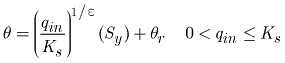
The specified infiltration rate is converted to water content in order to apply the characteristic solutions for unsaturated flow. A relation between water content and infiltration rate can be determined assuming the flux is equal to the unsaturated hydraulic conductivity using equations 2 and 14 (Charbeneau, 1984):
 ,
(19a)
,
(19a)
 ,
(19b)
,
(19b)
where
is |
the water content of a wave generated from infiltration, and |
|
is |
the infiltration rate (length per time). |
The water content is set to the saturated water content when the infiltration rate specified in the UZF1 Package input file exceeds the saturated vertical hydraulic conductivity. If the specified infiltration rate is greater than the saturated vertical hydraulic conductivity, then the difference is multiplied by the model cell plan-view area and this volumetric rate of water can be added to a user-specified stream reach or lake by setting the UZF1 Package variable IRUNFLG to greater than zero. Equation 19 ignores the time to ponding and infiltration rates that exceed the saturated vertical hydraulic conductivity (Smith and Parlange, 1978).
An algorithm was written in FORTRAN using equations 12, 14, 15, 16, 17, 18 and 19 to simulate vertical unsaturated flow and ET. This algorithm keeps track of the location, water content, velocity, and flux of all waves in the unsaturated zone through time and the interaction of waves overtaking one another. Additionally, changes in the thickness of the unsaturated zone owing to changes in the elevation of the water table are considered with respect to waves reaching the water table and contributing to ground-water storage.
Flow from the unsaturated zone as recharge to the water table in an unconfined aquifer is subtracted from the right-hand side of the system of equations that are solved by MODFLOW-2005:
 ,
(20)
,
(20)
where
is |
a matrix containing the coefficients of the conductance equations (HCOF array) that are solved by MODFLOW-2005; |
|
is |
a one-dimensional vector containing the ground-water heads that are solved by MODFLOW-2005; |
|
is |
a one-dimensional vector containing all known terms in the conductance equations that are not multiplied by unknown head values (RHS array); and |
|
is |
the volumetric rate (volume per time) of recharge computed in a given model cell from the UZF1 Package. |
Recharge that is simulated using the UZF1 Package is dependent on the water table elevation (ground-water head). Thus, the UZF1 Package is coupled to MODFLOW-2005 within the iteration loop. However, because ground-water recharge is dependent on the amount of storage and the downward flux rate in the unsaturated zone, there is no general equation that defines the relation between recharge and ground-water head, such as the conductance equation in the Streamflow-Routing (SFR1) Package (Prudic and others, 2004). Recharge from the UZF1 Package does not affect the HCOF array.
Based on the test simulations presented in this report, the UZF1 Package does not cause additional instabilities or slow convergence of MODFLOW-2005 when ground water is not discharging to land surface. Ground-water levels that rise above land surface add an additional head dependency when using the UZF1 Package owing to the calculation of ground-water discharge to land surface, and consequently, convergence may be slowed significantly when ground water is discharging to land surface from many model cells. MODFLOW-2005 simulations using the UZF1 Package may increase simulation time compared to using the Recharge Package owing to the additional calculations required to simulate flow through the unsaturated zone.
An infiltration rate at land surface (length per time) is specified for each vertical column in the active model domain (appendix 1). The infiltration rate is multiplied by the plan-view area of the cell to produce a volumetric flow rate (volume per time). Three options are used in the UZF1 Package to determine where flow in the unsaturated zone recharges ground water (UZF1 variable NUZTOP). The three options are those used in the Recharge Package (McDonald and Harbaugh, 1988, p. 7-6; Harbaugh and others, 2000, p. 67-68). The first option specifies that all recharge is to the top model layer only; the second option allows for recharge to be specified for a particular layer in each vertical column; and the third option allows for recharge to the uppermost active cell in a vertical column. When the last option is used in the UZF1 Package, the program will continue to route water through the unsaturated zone until it reaches the water table of the uppermost active cell. However, the hydraulic properties of the unsaturated zone will remain constant even if the unsaturated zone spans more than one cell in the vertical direction. If there are no active cells in a column beneath land surface, then infiltration and recharge do not occur and a warning statement is printed to the output file. If a cell becomes active during a simulation and the corresponding element in the UZF1 array IUZFBND is nonzero, then infiltration and recharge will start to occur.
As stated previously, mass balance is achieved by approximating the residual water content variable with the specific retention computed as the saturated water content minus the specific yield. Thus, if the water table rises into the unsaturated zone, the aquifer will yield an amount of water equal to the water table rise multiplied by the difference between the water content and the specific retention. Alternately, if the water table falls due to ground-water discharge or pumping at some other location, then the water content in the unsaturated zone between the old and new water table is set equal to the specific retention.
Recharge occurring during a rising water table over a time step is calculated by first routing waves through the unsaturated zone using the base of the unsaturated zone as the water-table elevation at the end of the previous time step. Flow across the base is accumulated for the time step and the volume of water in the unsaturated zone through which the water table rose over the time step is added to the volume that flowed past the base. This sum is divided by the time step to obtain a volumetric recharge rate. Once the flow equation has been solved for the time step, a new base of the unsaturated zone in each active cell is computed. Recharge occurring during a declining water table is computed based on the flux of water from the unsaturated zone during the time step using the base of the unsaturated zone predicted at the previous iteration or time step.
The UZF1 Package also allows for ground-water discharge to the land surface whenever the water table in a cell is higher than the land-surface elevation. The volumetric rate of ground-water discharge to land surface is calculated on the basis of the following equation:
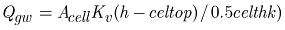 ,
(21)
,
(21)
where
is |
the water-table elevation; |
|
is |
the land-surface elevation; |
|
is |
the plan-view area of the model cell (equal to the column length times the row length of the model grid); |
|
is |
the vertical hydraulic conductivity of the model cell; and |
|
is |
the thickness of the model cell. |
The value that is subtracted from the HCOF array in
MODFLOW-2005 (corresponds to the A matrix in equation 20) is equal to ![]() .
The value subtracted from the RHS array in MODFLOW-2005 (corresponds to the
.
The value subtracted from the RHS array in MODFLOW-2005 (corresponds to the
![]() matrix in equation 20) is equal to
matrix in equation 20) is equal to ![]() .
.
The UZF1 Package includes an option to specify a two-dimensional array of values (UZF1 variable IRUNBND) that identify where ground-water discharge to land surface will be added to a stream or lake if the SFR2 and LAK Packages are active. Additionally, the UZF1 Package variable IRUNDFLG must be greater than 1 for water to be added to streams or lakes. Ground-water discharge to land surface and infiltration in excess of the saturated vertical hydraulic conductivity are added instantaneously to specified streams and lakes. The SFR2 Package is documented by Niswonger and Prudic (2006) and the LAK3 Package is documented by Merritt and Konikow (2000).
A water budget for the unsaturated zone is tracked independently of the ground-water budget within MODFLOW‑2005. The mass balance for the unsaturated zone accounts for all water between the land surface and the water table. The mass balance for the saturated zone is accounted for in the ground-water budget. When the water table rises above the top of a model cell, then the unsaturated-zone mass balance ceases to be calculated for that cell, and unsaturated storage and the change in unsaturated-zone storage for that cell are set to zero.
There are no procedural limitations regarding stress period and time step lengths associated with the UZF1 Package. However, because the UZF1 Package delays recharge to the water table, changes in stress do not necessarily correspond to the beginning of a stress period. Consequently, caution should be used when simulating time steps that increase during a stress period (specifying the variable TSMULT>1.0 in the data input for the Discretization file; Harbaugh, 2005) because water percolating through the unsaturated zone may reach the water table at the end of a stress period, when the time step length is a maximum.
Steady state can be specified for the initial stress period of a simulation when using the UZF1 Package. When steady state is specified for the initial stress period, the ground-water recharge rate computed in UZF1 is set equal to the infiltration rate and ET is not removed from the unsaturated zone. The water content is constant within each model cell during steady state. The specified ET rate is subtracted from the infiltration rate to calculate a steady-state recharge rate. ET can also occur from ground water when the water table is above the ET extinction depth. A uniform water content profile is computed for each active cell, which is used automatically as the initial conditions for a following transient stress period.
Steady-state water content profiles may be printed to a file for specified locations. Initial water content values are not required when the initial stress period is specified as steady state. Thus, initial water-content values must not be specified within the UZF1 input file when the first stress period is steady state. Another option for developing initial water content profiles is to run the model for several years while repeating a cycle of infiltration rates. This step may be carried out subsequent to a steady-state simulation.
The kinematic-wave approximation does not account for capillary-induced infiltration at the onset of wetting when negative pressure gradients are large relative to gravity potential gradients. However, infiltration approaches the unsaturated hydraulic conductivity when the wetting front has advanced sufficiently far beneath the surface (Mein and Larson, 1973; Childs and Bybordi, 1969). Negative pressure gradients also may result in lateral and vertical redistribution in the unsaturated zone. Because negative pressure gradients are ignored, UZF1 likely under predicts the advancement of the wetting front at early times.
Because capillary-induced infiltration is neglected, there is no consideration for the period prior to ponding when the infiltration should be represented by a constant flux equal to the rainfall rate (Smith and Parlange, 1978), rather than the constant water content assigned at the boundary (equation 19). Thus for greater rainfall or snowmelt rates, the model will underestimate infiltration during the onset of infiltration. UZF1 does not simulate a capillary fringe above the water table and it assumes that ground water is instantaneously released from or taken into storage.
The initial version of this package (UZF1) does not simulate unsaturated flow through multiple layers of varying hydraulic properties. The model can simulate unsaturated flow through inactive cells to deeper active model cells. However, the hydraulic properties of an unsaturated column between the land surface and the uppermost active cell are uniform during the simulation and are always equal to their values at the onset of the simulation.

![]() U.S.
Department of the Interior | U.S. Geological
Survey
U.S.
Department of the Interior | U.S. Geological
Survey
Persistent URL: https://pubs.water.usgs.gov/tm6a19
Page Contact Information: Publications Team
Page Last Modified: Friday, 02-Dec-2016 15:45:18 EST
