
Techniques of Water-Resources Investigations 8-A3
BASIC PRINCIPLES OF PRESSURE AND PRESSURE MEASUREMENT
PRESSURE TRANSDUCER CHARACTERIZATON
PLANNING CONSIDERATIONS FOR SENSOR SYSTEMS
ASSEMBLY, CALIBRATION, AND TESTING
APPLICATIONS TO WATER-RESOURCES INVESTIGATIONS
TECHNIQUES OF WATER-RESOURCES INVESTIGATIONS OF THE U.S. GEOLOGICAL SURVEY
Figure 1. Relation between force and pressure for an unconfined unit liqui...
Figure 2. Relation between force and pressure for a confined fluid at rest...
Figure 3. Differences between absolute pressure and gage pressure.
Figure 4. Resistors in a series.
Figure 5. Resistors in parallel.
Figure 6. Mixed-circuit analysis.
Figure 8. Wheatstone bridge with input shorted.
Figure 9. Thevenin equivalent circuit.
Figure 10. Graph used for computing minimum parallel and maximum series re...
Figure 11. Graph showing envelope of minimum parallel and maximum series r...
Figure 12. Examples of different types of force-summing devices.
Figure 13. A piezoelectric pressure transducer using a diaphram as a force...
Figure 14. A capacitive pressure transducer using a bellows as a force-sum...
Figure 15. An inductive (active) pressure transducer using a diaphram as a...
Figure 16. A reluctive (passive) pressure transducer using a Bourdon tube ...
Figure 17. A potentiometric pressure transducer and resistance-measuring c...
Figure 18. A vibrating wire pressure transducer (modified from CEC Instrum...
Figure 19. A vibrating cylinder pressure transducer (modified from CEC Ins...
Figure 20. An unbonded strain gage.
Figure 21. A bonded strain gage (modified from CEC Instruments, no date).
Figure 22. Electrical schematic of a compensated Wheatstone bridge.
Figure 23. Illustration of zero drift and sensitivity.
Figure 24. Illustration of zero error.
Figure 25. Illustration of span error.
Figure 26. Illustration of nonlinear error.
Figure 27. Illustration of error band.
Figure 28. Illustration of hysteresis.
Figure 29. Illustration of resolution.
Figure 30a. Illustration of sensitivity.
Figure 30b. Illustration of sensitivity.
Figure 31. Illustration of time constant.
Figure 32. Housing for low-cost pressure transducer with a thermistor.
Figure 33. Housing for low-cost pressure transducer.
Figure 34. Input-current loading error.
Figure 35. Shunt-resistance loading error.
Figure 36. Voltage-burden error.
Figure 37. Two-wire configuration.
Figure 38. Four-wire configuration.
Figure 39. Equipment used for temperture-corrected transducer calibration.
Figure 40. Shelter design for a pressure-transducer installation.
Figure 41. Submersible transducer in an observation well.
Figure 42. Example calibration worksheet for submersible transducers.
Figure 43. Ground-water inspection sheet.
Figure 44. Ground-water record station analysis.
Figure 45. Drain-cleaner packer.
Figure 46. Drop-pipe protection of a submerged transducer.
Figure 47. Surface-water monitoring installation.
Figure 48. Soil-water tensiometer.
Figure 49. Field tensiometer installation.
Figure 50. Pressurized housing for pressure transducer.
Figure 51. Housing for cable splice.
CONVERSION FACTORS, VERTICAL DATUM, AND ABBREVIATIONS
Table 1. Pressure-unit conversion factors.
Table 2. Conversion of measurement precision in percent to decades.
The terms in this glossary were compiled from numerous sources. Some definitions have been modified in accordance with usage of submersible pressure transducers for ground-water-level monitoring and may not be the only valid definitions for these terms.
Absolute Pressure Transducer: A pressure transducer that has an internal reference chamber sealed at or close to 0 psi absolute (full vacumn).
Accuracy (absolute): A measure of the closeness of agreement of an instrument reading compared to that of a primary standard having absolute traceability to a standard sanctioned by a recognized standards organization. This definition of accuracy is rarely used in manufacturer's specifications.
Accuracy (relative): The ratio of the error of an instrument reading to the full-scale output of the instrument or the ratio of the error to a specified output expressed as a percent. Normally this statement of accuracy will include the effects of non-linearity, hysteresis, and repeatability. This definition of accuracy is most commonly used by manufacturers.
Analog output: Transducer output that is a continuous function of the measurand (value of the physical property) as distinguished from digital (discrete) output.
Best-fit straight line: A line chosen to represent the sensitivity of a transducer; from it non-linearity errors may be calculated. The best-fit straight line may be determined from a least-squares linear regression fit of the measurand input and transducer output.
Bridge circuit: An instrument for measuring electrical values by comparing the unknown value with known values. When all values are equal the bridge is said to be 'balanced' or 'nulled'.
Burst pressure: The specified maximum pressure that may be applied to the sensing element of the transducer without rupture of either the sensing element or the transducer case.
Compensation: Provision of a supplemental device, circuit, or special material to counteract known sources of error such as temperature, shock, and vibration.
Creep: A change in output occurring over a specific time period while the measurand and all environmental conditions are held constant.
Data logger: An electronic digital data recorder used by engineers, scientists, and technicians.
Dead volume: The total volume of the pressure port cavity of a transducer under room temperature and barometric pressure.
Diaphragm: The force-sensing membrane that is deformed when pressure is applied.
Digital output: Transducer output that represents the magnitude of the measurand in the form of a series of discrete quantities, coded in a system of notation, as distinguished from analog output.
Drift: A change in output over a period of time that is not a function of the measurand (measured property). Drift is normally specified as a change in zero (zero drift) over time and a change in sensitivity (sensitivity drift) over time.
Error: The algebraic difference between the indicated value and the true value of the measurand.
Error band: The band of maximum deviation of output values from a specified calibration curve or reference line.
Excitation: The external electrical voltage or current applied to a transducer for its operation, usually expressed as a range of voltage or current values.
Force-sensing device: The diaphragm and associated mechanical components that move and cause a change in position that can be sensed by the electrical components in a transducer.
Full-scale output: The algebraic difference between the outputs at the specified upper and lower limits of the measurand inputs.
Gage transducer: A transducer that measures pressure relative to the ambient atmospheric pressure.
Hysteresis: The maximum difference in output, at any measurand value within the specified range, when the value is approached first with an increasing and then with a decreasing measurand. Hysteresis is expressed in percent of full-scale output.
Inductive transducer: A transducer in which the mechanical movement is converted to an electrical signal through electrical induction.
Linearity: The closeness of a calibration curve to a specified straight line. Linearity is expressed as a percent of the full-scale output using the maximum deviation of any calibration point from a specified straight line.
Mean time between failures (MTBF): The total time that a number of sensors operate divided by the number of sensors that fail during the operational period. A value of MTBF usually characterizes a single type of component or a production batch from one manufacturer.
Measurand: The value of the physical property being measured.
Precision: The ability to reproduce output readings when the same measurand is applied, consecutively, under the same conditions, and in the same direction. Precision is a measure of the repeatability of a measurement. Precision does not imply accuracy. If a measurement system has good repeatability, then consecutive readings will be densely grouped together when the readings are plotted.
Pressure-sensing system: As used in this report, a pressure-sensing system is composed of a data recorder, pressure transducer, electrical connections, power supply, atmospheric pressure sensor or vent tube, and the transducer suspension apparatus.
Pressure transducer: A type of measurement device that converts pressure-induced mechanical changes into an electrical signal.
Proof pressure: The maximum pressure that may be applied to the sensing element of a transducer without changing its performance beyond the specified tolerances.
Range: The upper and lower limit of the measurand within which a transducer is intended to measure.
Reference pressure: The pressure to which a differential pressure transducer measurement is compared.
Reliability: The probability that an item will perform its intended function for a specified interval under stated conditions.
Resolution: The smallest change in the measurand that can be measured or detected in the output reading.
Response time: The length of time required for the output of a transducer to rise to a specified percentage of its final value as a result of a step change in the measurand.
Shunt resistor: A precision resistor with a known value that is used to calibrate a pressure transducer.
Sensitivity: The ratio of the change in transducer output to a change in the measurand. Sensitivity may vary over the operational range of the transducer.
Specific Gravity: The ratio of the mass of a body to the mass of an equal volume of water at 4 °C or other specified temperature.
Stability: The ability of a transducer to retain its performance characteristics for a period of time. Stability is normally expressed in percent of full-scale output over a set period of time.
System effectiveness (reliability): The probability that a system can successfully meet an overall operational demand within a given time when operated under specified conditions.
Test envelope: A line or lines bounding the measured values on a graph of true values versus measured values of a single property (for example, pressure).
Time constant: The length of time required for the output of a transducer to rise to 63 percent of its final value as a result of a step change in the measurand.
| Multiply | By | To obtain |
|---|---|---|
| inch (in.) | 25.4 | millimeter |
| square inch (in.2) | 6.452 | square centimeter |
| foot (ft) | 0.3048 | meter |
| pounds (lbs) | 0.4536 | kilogram |
Temperature:
Water and air temperature are given in degrees Celsius
(°C), which can be converted to degrees Fahrenheit
(°F) by use of the following equation:
°F = 1.8 (°C) + 32
Absolute temperature
in degrees Kelvin (°K) can be converted to degrees
Celsius (°C) by use of the following equation:
(°C) = (°K) − 273.15
Sea level: In this report "sea level" refers to the National Geodetic Vertical Datum of 1929 (NGVD of 1929)—a geodetic datum derived from a general adjustment of the first-order level nets of both the United States and Canada, formerly called Sea Level Datum of 1929.
AC - alternating current
DBLS - depth below land surface
DC - direct current
EDL - electronic data logger
EMF - electromotive force
FPS - foot-pound-second measurement system
Hg - mercury
H2O - water
lbs/in.2 - pounds per square inch
MKS - meter-kilogram-second measurement system
MTBF - mean time between failures
mV - millivolt
µV - microvolt
N - Newtons
Pa - Pascals
psi - pounds per square inch
PVC - polyvinyl chloride
USGS - U.S. Geological Survey
V - volt
Submersible pressure transducers, developed in the early 1960s, have made the collection of water-level and pressure data much more convenient than former methods. Submersible pressure transducers, when combined with electronic data recorders have made it possible to collect continuous or nearly continuous water-level or pressure data from wells, piezometers, soil-moisture tensiometers, and surface water gages. These more frequent measurements have led to an improved understanding of the hydraulic processes in streams, soils, and aquifers.
This manual describes the operational theory behind submersible pressure transducers and provides information about their use in hydrologic investigations conducted by the U.S. Geological Survey.With the improvement of instruments used to collect and record ground-water level data, provision of consistent guidelines for the use of this equipment is important to those who collect the data. Submersible pressure transducers (pressure-sensing devices) and electronic data loggers (digital data recorders) have become an integral part of U.S. Geological Survey (USGS) hydrologic investigations that collect time-series data on water-level fluctuations in wells. Because of the perceived ease of installation and operation of submersible pressure transducers and data loggers, data provided by these systems commonly are not adequately supported by quality-assurance procedures and documentation. Submersible pressure transducers occasionally are misused, either because of a lack of understanding of the capability of a particular transducer, or because of a lack of attention to its calibration and maintenance. This manual describes the operational theory fundamental to all transducers and provides detailed information about the use of submersible pressure transducers in hydrologic investigations conducted by the USGS.
Electrical pressure transducers designed to be immersed in water (submersible pressure transducers) have been used by ground-water scientists since the early 1960s (Shuter and Johnson, 1961; Garber and Koopman, 1968). These pressure-sensing devices, typically installed at a fixed depth in a well, sense the change in pressure against a membrane. Pressure changes occur in response to changes in the height, and thus in the weight of the water column in the well above the transducer. Substantial improvements in design, operation, and accuracy of electronic submersible pressure transducers and data recording systems have led to a significant increase in their use, replacing older systems (described in the box) in some applications.
Submersible pressure transducers also are used to monitor surface water elevations (Meyers, 1994) and variations in soil moisture tension in the unsaturated (vadose) zone (Healy and others, 1986). Several types of water-level sensors can provide time-series data to an electronic data logger, but for many applications only submersible pressure transducers are suitable (Freeman, 1996). Because many types of submersible pressure transducers are available, it can be difficult to determine which type is most appropriate for a particular hydrologic investigation or application.
Early systems that recorded continuous water-level changes in wells consisted of a float connected to a steel tape or beaded cable and a counterweight connected to a wheel. The rotating wheel turned a drum, upon which a pen, connected to a clock, recorded water levels on a paper chart. Another system, in use since the 1960s, uses an electrical device to sense the water surface in a well, either with a series of electrodes or with a membrane deflected by the water surface. These probes control an electrically activated drum located at the top of the well. The drum rotates either clockwise or counterclockwise until the sensor is situated at the water surface. The data are recorded on a continuous paper chart or by a digital recorder. A third type of sensor that has been in use since the early 1980's is an acoustic velocity device such as the Polaroid acoustic distance-measuring device. It measures the changes in depth to the water surface by measuring the variations in elapsed time between sending and receiving sound waves.
This manual is intended to be a guide to the proper selection, installation, and operation of submersible pressure transducers and data loggers for the collection of hydrologic data, primarily for the collection of water-level data from wells. The manual describes the basic principles, measurement needs, and considerations for operating submersible pressure transducers, including a discussion of the systematic errors inherent in their use. Standard operational procedures for data collection and data processing, as well as applications of transducers for specific types of hydrologic investigations are included. Basic concepts regarding the physics of pressure and the mechanics of measuring pressure are presented, along with information on the electronics used to make and record these measurements. Guidelines for transducer calibration, proper use, and quality assurance of data also are presented. Field applications of pressure transducer systems are discussed for ground water, surface water, and the unsaturated zone; as are common problems that may corrupt data, and suggestions for field repairs.
The physics of pressure and types of pressure measurements described in this section provide the background understanding for the application of pressure transducers to hydrologic investigations. An overview of the basic principles of direct current (DC) circuits is provided, since an understanding of the operational theory behind sensing and recording systems requires a working knowledge of DC circuitry. The application of these principles and operations to measure pressure with pressure transducers is addressed in later sections of this manual.
Pressure (P) is defined as the force (F) exerted per unit of surface area (A) over which the force is applied. In classical mechanics, when two solid objects are in contact with each other, the pressure exerted by one object on another object is defined as:
P = dF/dA, (1) where:
dF = force or weight (mass x acceleration)
acting on the contact surface and
dA = contact area over which the force is applied.
In fluid mechanics, pressure is similarly defined. For purposes of this discussion, fluid refers to both liquids and gases. Unlike solids, however, fluids possess negligible shear strength and will completely or partially occupy the volume of the container in which they are placed. A liquid, if it does not completely fill the container, will present a free liquid surface. A gas, on the other hand, will always fill the volume of its container.
When a gas is confined in a container, molecules of the gas strike the walls of the container. The collision of the molecules against the container walls results in a force exerted against the surface area of the container. Pressure in the container is this force divided by the surface area of the container. Pressure within the container is the same everywhere. For a given mass of gas, pressure inside a container will vary in response to changes in the volume of the container and in the temperature of the gas in accordance with the relations expressed in the combined (Charles's and Boyle's) gas law:
PV = constant x T (2)
(for a given gas, the volume is inversely
proportional to the pressure and directly
proportional to the absolute temperature),
and in the ideal gas law:
PV = nRT, (3) where:
P = pressure,
V = volume,
n = moles of gas (mass),
R = universal or molar gas constant, and
T = temperature
The pressure at a point in a gas that is not confined to the volume of a container, and is at rest, such as atmospheric air, is dependent upon the density and height of the column of gas above the point of measurement. Because gas is compressible, its density will vary in response to position or elevation. Temperature differences, in an otherwise static column of air, also will affect gas densities. For example, atmospheric pressure decreases with increasing altitude; the relationship is not linear, however, because air density and temperature also decrease with increasing altitude. Gas pressure exerted at a point is identical in all directions around the point of measurement.
For a liquid at rest that is not confined, the pressure exerted by the liquid at any point depends upon the density and the height of the column of liquid above the point of measurement. Because water is only slightly compressible, its density can be assumed to be constant, provided temperature and salinity do not vary significantly above the point of measurement. Pressure at any point in a liquid acts perpendicularly against the surfaces it contacts. Within the liquid, the pressure at a point is identical in all directions from the point of measurement. This principle is illustrated in the use of open-ended manometers to measure pressure differentials as shown in figure 1.
In figure 1, pressure P1 is greater than P2 by an amount equal to the height (h) of fluid in the manometer times the specific gravity of the fluid. In the absence of capillary forces, the diameters of the reservoir (D) and manometer (d) have no influence on the differential height of fluid between the two liquid surfaces.
Figure 1. Relation between force and pressure for an unconfined unit liquid at rest.
Whenever an external pressure is applied to a confined fluid at rest, either liquid or gas, the pressure increases at every point in the fluid by the amount of the external pressure applied. This principle, known as Pascal's law, is the basis for the design of the hydraulic lift, closed-end manometers, and many other types of pressure-sensing or transduction devices. This principle is illustrated in figure 2.
In figure 2, a downward force (F) of 100 pounds (lbs) acting across an area of 1 square inch (in2) produces a pressure (P) of 100 pounds per square inch (lbs/in2 or psi). Because the fluid is confined, pressure is the same throughout the fluid, regardless of position. The downward applied force of 100 lbs produces an equivalent force of 5,000 lbs when the pressure is transmitted across an area of 50 in2. Unlike the example of the unconfined fluid system shown in figure 1, fluid displacement is dependent on the size of the reservoirs and tubes. Mechanical advantage is gained by difference in the area of the pistons.
Figure 2. Relation between force and pressure for a confined fluid at rest.
Pressure may be expressed in any one of the three major systems of units. The standard unit of pressure in the English, or foot-pounds-second (FPS), system is pounds per square inch, abbreviated as psi. In the meter-kilogram-second (MKS) system of measurement, pressure is expressed as kilograms per square meter. In standard international (SI) units, pressure is expressed in Newtons (N) per square meter, or Pascals (Pa).
In ground-water hydrology, the length unit of measurement commonly is used to represent pressure because it is easily referenced to the total energy at a point in the ground-water flow system. The total energy at a point in a body of water equals the sum of its potential energy and kinetic components. For any incompressible fluid, either at rest or in motion, this relation is expressed as:
| h = | P/γ + z | + | v2 / 2g | (4) |
| potential energy | kinetic energy |
where:
h = total energy potential, or head,
P = pressure,
γ = density of fluid,
z = position potential or elevation with respect to a
specified datum,
v = velocity, and
g = acceleration of gravity
Total energy potential or head is simply the summation of position (z) above or below some reference or elevation datum, height of the column of water above the point of measurement, and a kinetic energy term expressed in units of length. In most ground-water hydrology applications, velocity (v) is very nearly zero and the kinetic energy term is therefore assumed to be zero. Because pressure in a static water body is determined by the height of the column of water above the point of measurement, it is convenient to express pressure in units of length. At the water surface, pressure head is zero and total head (or potential) is simply the height of the water surface above or below the reference datum. In ground-water hydrology, potential commonly is referred to as "head." In the FPS system, it is expressed in terms of feet or inches of water; in the MKS system, as meters or centimeters of water.
Pressure-unit conversion factors commonly used in hydrology are listed in table 1. Take care when applying these conversion factors. Pressure expressed in terms of mercury (Hg) or water (H2O), for example, depends on the specific gravity or density of the fluid, which is temperature dependent. In the case of water, the effects of total dissolved solids and suspended solids (turbidity) on density also must be considered when quoting pressure head in terms of length.
Table 1. Pressure-unit conversion factors.
| Multiply | FPS lb/in2 | MKS kg/m2 (1) | SI N/m2 (pascal) | Temperature Specification |
|---|---|---|---|---|
| lb/in.2 (psi) | 1 | 1.422 x 101 | 6.895 x 10 3 | |
| ft of H2O | 4.336 x 10⁻¹ | 3.048 x 10 2 | 2.989 x 10 3 | 4°C |
| in of Hg | 4.912 x 10 -1 | 3.453 x 10 2 | 3.377 x 10 3 | 0°C |
| mm of Hg | 1.934 x 10⁻² | 1.359 x 10 -3 | 1.333 x 10 2 | 0°C |
| atmosphere (atm) | 1.470 x 101 | 1.033 x 10 4 | 1.013 x 10 5 | |
| N/m2 (Pascal) | 1.450 x 10 - 4 | 1.020 x 101 | 1 | |
| bar | 1.450 x 101 | 1.020 x 10 4 | 1.000 x 10 5 | |
| kg/m2(1) | 1.422 x 101 | 1 | 9.807 | |
| (1) One kilogram mass under standard gravitational acceleration. | ||||
Absolute pressure is measured in reference to a vacuum or zero pressure. Pressure at sea level is 1 atmosphere, 101.3 kPa, or 14.70 psi. Pressures measured by an absolute pressure transducer are always positive because these devices are referenced to a perfect vacuum in which absolute pressure is zero. Zero referencing is accomplished by completely evacuating and sealing the interior or reference side of the transducer.
Gage pressure is measured in reference to atmospheric pressure at mean sea level. Pressures measured by a gage-pressure transducer are positive for pressures greater than sea-level pressure and negative for pressure less than sea-level pressure. Thus, atmospheric pressure measurements above sea-level datum are negative because atmospheric pressure decreases with altitude. Sea-level referencing is accomplished by sealing the interior or reference side of the transducer to atmospheric pressure at sea level. The term "gage pressure" is sometimes used to describe pressure measurements referenced to ambient atmospheric pressure other than to sea level. The relation between absolute pressure and gage pressure is illustrated in figure 3.
Figure 3. Differences between absolute pressure and gage pressure.
Differential pressure is measured with respect to a varying pressure reference such as ambient atmospheric pressure or some other pressure source that is allowed to vary independently of the primary measurement. Pressure transducers constructed in this manner actually sense the difference between two independent pressure sources simultaneously. The output of the differential pressure transducer is proportional to the pressure difference between the two independent sources. Pressure measurements made with open-ended manometers or vented submersible pressure transducers are examples of differential measurements.
Sealed-reference pressure is measured with respect to a sealed reference pressure other than atmospheric pressure at sea level. A sealed-reference pressure is created by evacuating (pressuring down) or pressuring up the interior or reference side of the transducer to a prescribed absolute pressure. Because the sealed-reference side contains a constant volume of gas, the transducer must be maintained at a constant temperature to avoid changes in the reference pressure.
The most common type of pressure transducer is the strain-gage pressure transducer. Understanding the operational theory behind these transducers requires a working knowledge of basic DC circuitry. This knowledge applies as well to the operation of the electronic components used to excite and read the device. Many problems encountered in the field can be analyzed and diagnosed by applying some simple techniques that require a working knowledge of DC circuitry. In the following illustrations, V is voltage, I is current, and R is resistance.
The overview of DC circuit analysis illustrates how a DC circuit can be reduced to an equivalent single voltage source and a single resistor. For example, in the top part of figure 4, a circuit consists of a battery and two resistors, R1 and R2, in series. The battery supplies a voltage (V) causing a current (I) to flow in the circuit. Each resistor produces a voltage drop (V1 and V2). Current flow is continuous through the circuit, so I = I1 = I2. The total resistance of the circuit is the sum of the individual resistances (R = R1 + R2); therefore the circuit in the lower part of figure 4 is functionally the same as the circuit in the top part.
V = IR
(Ohm's law)
R = R1+ R2...+ Rn
(resistance is additive)
I = I1 = I2 = In
(current is constant across each resistor)
V = V1 + V2 ... + Vn
(voltage drops are additive)
V = I (R1+ R2...+ Rn)
(voltage divides in proportion to resistance)
Figure 4. Resistors in a series.
For resistors in parallel, the voltage drop across each resistor is the same (V = V1 = V2). From Ohm's Law, V1 = I1R1 and V2 = I2R2, so I1R1 = I2R2 and the total current flow in the circuit is the sum of the current in each branch (I = I1 + I2). Because I1 = V/R1 and I2 = V/R2, I=V/R1+V/R2 and I=V/R as shown in the lower part of figure 5.
V = IR
(Ohm's law)
1/R = 1/R1 + 1/R2...+ 1/Rn
(the reciprocal of resistance is the sum of the reciprocals of each resistance)
R = R1R2
R1+ R2
(special case for two resistors in parallel)
I = I1 + I2 ... + In
(current is proportional to resistance)
V = V1 = V2= Vn
(voltage is constant across each resistor)
Figure 5. Resistors in parallel.
For multiple parallel and series components the procedure is virtually the same. First, convert independent or isolated parallel components to an equivalent resistor, then convert any resulting series components to an equivalent resistor. Repeat this process until all resistors are reduced to one equivalent resistor as shown in the box and in figure 6.
Figure 6. Mixed-circuit analysis.
Convert the mixed circuit in figure 6 to a single
voltage source and resistor and find I, I1, I2, Ia, Ib,
V1,V2,Va, Vb, Rc, and Reqv
Given:
V = 10 volts
R1 = 91 ohms R2 = 100 ohms
Ra = 90 ohms Rb = 10 ohms
Convert parallel-bRanch component to an
equivalent resistor, Rc
1/Rc = 1/Rb + 1/Ra
Rc = (RbRa)/(Rb + Ra) = 900/100 = 9 ohms
Convert series resistors to an equivalent resistor
Reqv = R1 + R2 + Rc = 91 + 100 + 9 = 200 ohms
1. Compute I, I1, I2, Ic
I = V/Reqv = 10 volts/200 ohms = 0.05 amps
I = I1 = I2 = Ic = 0.05 amps
2. Compute V1, V2, Vc
V1 = IR1 = (0.05 amps x 91 ohms) = 4.55 volts
V2 = IR2 = (0.05 amps x 100 ohms) = 5.00 volts
Vc = IRc = (0.05 amps x 9 ohms) = 0.45 volts
V = V1 + V2 + Vc = 10.0 (volts check)
3. Compute Va, Vb, Ia, Ib
I = I1 = I2 = Ia + Ib
Vc = Va = Vb = 0.45 volts
Ia = Va /Ra = 0.45/90 = 0.005 amps
Ib = Vb /Rb = 0.45/10 = 0.045 amps
I = Ia + Ib = 0.05 amps (check)
Complex resistance circuits cannot be broken down into a simple equivalent resistor. More complex DC circuits require the application of Kirchhoff's laws to analyze the separate components of the circuit. Kirchhoff's laws state:
An example of a circuit requiring the application of Kirchhoff's laws is the Wheatstone bridge, variations of which are used in many strain-gage pressure transducers (for example, in the common bonded-foil strain-gage transducers). The Wheatstone bridge circuit (fig. 7) consists of four resistors (R1 through R4) supplied with a fixed voltage (Vin). When all resistances are equal, the current through each resistor is equal (I1= I2= I3= I4) and no voltage difference is measured at the voltmeter (V). The bridge is then said to be 'balanced.'
Step 1: With the input voltage source shorted, reduce the circuit to an equivalent resistance (RS) as seen across the open circuit (or output voltage leads) shown in figure 8.
Given:
Vin = 10 volts
R1 = 2000 ohms
R2 = 2000 ohms
R3 = 1900 ohms
R4 = 2000 ohms
With the input voltage shorted, the circuit reduces to two parallel branches that are in series, as seen across the output voltage leads (VS). Circuit simplification reduces each parallel component to an equivalent resistor followed by adding in series:
| RS = | R1R2 | + | R3R4 |
| R1+ R2 | R3+ R4 |
RS = 1974.36 ohms
Step 2: Determine the open-circuit voltage (VS) appearing across the output voltage leads using the input voltage (Vin). Determine voltage potential (VS) across the output leads, where:
VS = I2R2 - I3R3 = I1R1 - I4R4
Iin = I2 + I3
(Kirchhoff's first law)
I2R2 + I1R1 = I3R3 + I4R4
Vin = I3R3+ I4R4
(Kirchhoff's second law)
I1 = I2, I3 = I4
(current is constant across resistors in series)
10V = 1500 I3 + 2000 I4Compute I1 and I2
10V = 3900 I4
I4 = 2.5641 milliamps = I3
10V = 2000 I1 + 2000 I2Compute short-circuit current
10V = 4000 I2
I2 = 2.5 milliamps = I1
VS = I2R2 - I3R3 = 128.2 millivolts
IS = VS/RS = 0.065 milliamps
The Thevenin equivalent circuit for the example Wheatstone bridge is shown in figure 9.
Understanding DC circuits can be an invaluable aid in error analysis, selecting measurement instruments, optimizing pressure transducer performance, and troubleshooting system malfunctions. Circuit analysis can be applied to test for electrical short circuits, to locate damaged bridge elements, or to find insulation leakage in the circuit.
A Thevenin equivalent circuit is a hypothetical circuit designed to simplify the analysis of complex, two-terminal linear networks, such as Wheatstone bridges. Thevenin's theorem states that any potential source that has only two output terminals and is composed of resistors and a voltage or battery source can be represented by a series combination of a resistor (RS) and voltage source (VS) as shown in figure 9. VS is the open-circuit potential and Rs is the resistance between the output terminals when the battery or voltage source is shorted. The equivalent circuit is constructed by applying Ohm's law to parallel and series components in the network, reducing the circuit to a voltage source (VS) connected in series with a Thevenin equivalent resistance (RS). The procedure for constructing a Thevenin equivalent circuit for the common Wheatstone bridge is described on the preceding page.
Figure 8. Wheatstone bridge with input shorted.
Figure 9. Thevenin equivalent circuit.
Constructing the Thevenin equivalent circuit is the first step in evaluating the adequacy of the measurement system to provide the necessary resolution and sensitivity to resolve the measurement of interest. Resolution and sensitivity are discussed in greater detail later in this manual. Once the expected signal levels (open circuit voltage and short circuit current) are defined, probable error sources that may affect the measurement can be identified. The application and value of this error analysis is illustrated by constructing what is referred to as a test envelope for the type of measurement (voltage, current, or resistance) being made. For purposes of illustration, the Wheatstone bridge in the example above will be used to construct the test envelope.
Construction of the test envelope is accomplished with reference to figure 10 and table 2. Determine the required measurement precision, which is 0.1% (1,000 parts per million) in this example; and determine the associated number of decades (table 2). The number of decades in this example is three. A decade is equivalent to one order of magnitude difference in the open-circuit voltage or short-circuit current. In figure 10, plot the computed open-circuit voltage (VS = 128 millivolts) and short-circuit current (IS = 0.065 milliamps). Extend a line the length of the number of decades – scaled to either the horizontal or vertical axis – vertically downward and extend a line of the same length horizontally to the left. Construct an arc the length of the total number of decades connecting the horizontal and vertical axes. The resulting envelope, shown in figure 11, defines the minimum values of resistance that can be placed in parallel with the Thevenin equivalent resistance (about 5 MΩ) and the maximum resistance that can be placed in series (about 5 Ω) without affecting the desired measurement precision. All resistance within the envelope, whether in parallel or in series, would seriously degrade the measurement. A second envelope is shown in figure 11 to illustrate the effect of increasing the measurement precision requirement from 0.1% to 0.01% (100 parts per million). In the second case, the minimum resistance in parallel is 50 MΩ, and the maximum resistance in series is 500 mΩ (0.5 Ω). Potential sources of errors due to parallel and series resistance in the measurement circuit are described in the section "Sources of Error When Making Direct Current Measurements."
| Percent | Parts per million | Decades |
|---|---|---|
| 10 | 100,000 | 1 |
| 1 | 10,000 | 2 |
| 0.1 | 1,000 | 3 |
| 0.01 | 100 | 4 |
| 0.001 | 10 | 5 |
Pressure transducers are characterized by their mechanical and electrical transduction elements, the performance specifications of the transducer, and the interaction of the transducer with the other components of the measuring system (such as the power supply and data logger).
A transducer is a device that converts energy from one form to another. Electrical pressure transducers, which measure changes in pressure, consist of a mechanical-transduction element or force-summing device coupled to an electrical-transduction element, which is connected to a display or recording device, or both. There are two types of electrical transduction elements—active and passive. Electrical-transduction elements that convert pressure-induced mechanical changes directly to an electrical signal are referred to as active transducers. Passive transducers require an external excitation that causes the transducers to respond to pressure-induced mechanical changes. The electrical-transduction element converts mechanical energy into electrical energy and the force-summing device or mechanical-transduction element converts gas or liquid energy into mechanical energy.
Many types of pressure transducers consist only of mechanical-transduction elements. Open-ended and closed-ended manometers, barometers that record changes in the height of a column of liquid in response to some external pressure change, and spring-loaded pressure-sensing devices are examples of mechanical transducers.
Electrical pressure transducers are classified primarily on the electrical principle or method of electrical transduction involved in their operation. Different electrical transduction elements can be coupled to a variety of force-summing devices. Some combinations work better than others, depending on the application and measurement needs. Commonly used types of force-summing devices are illustrated in figure 12. A piezoelectric pressure transducer incorporating the diaphragm in the housing is illustrated in figure 13.
Figure 12. Examples of different types of force-summing devices.
Figure 13. A piezoelectric pressure transducer using a diaphram as a force-summing device.
Electrical pressure transducers using force-summing devices are described below. The most common of the many types of pressure transducer is the strain-gage pressure transducer.
The piezoelectric transducer is an example of a self-generating or active pressure transducer. The design of this type of transducer is based on the ability of certain crystals (quartz, tourmaline, Rochelle salt, or ammonium dihydrogen phosphate) and ceramic materials (barium-titanate, or lead-zirconate-titanite) to generate an electrical charge or voltage when mechanically stressed. The crystal geometry of these materials is oriented to provide maximum piezoelectric response in one direction and minimal response in other directions. The transducer develops a voltage proportional to the change in pressure. These transducers cannot be calibrated using normal static-pressure calibration techniques. This type of transducer is used to measure rapidly fluctuating pressures.
In an inductive transducer, pressure-induced displacements of a diaphragm cause a change in the self-inductance of a single coil. In a reluctive transducer, displacements occur in the magnetic coupling between a pair of coils. An inductive transducer is active and operates on the principle that the relative motion between a conductor and a magnetic field induces a voltage in the conductor (fig. 15). Because the pressure-induced electrical output signal requires relative motion, the inductive design is limited to dynamic measurements. In a reluctive transducer, displacements occur in the magnetic coupling between a pair of coils. A reluctive transducer is passive and requires external AC excitation of a pair of coils. It operates on the principle that the magnetic coupling between the two coils is affected by the displacement of a pressure-driven conductor located in the magnetic field between the two coils. The conductor is either connected to a force-summing device or is itself a force-summing device. Two basic designs have evolved (figs. 15 and 16).
Figure 15. An inductive (active) pressure transducer using a diaphram as a force-summing device.
Figure 16. A reluctive (passive) pressure transducer using a Bourdon tube as a force-summing device.
The potentiometric pressure transducer consists of a movable contact driven by an active force-summing device (fig. 17). The movable contact, or wiper, travels across a resistive element that may be a wire-wound coil, a carbon ribbon, or a deposited conductive film. The motion of the wiper across the resistive element causes a change in the resistance selected by the wiper. The change in resistance produces an electric signal (either a change in voltage or current) that is proportional to the mechanical displacement of the wiper. This type of transducer may be excited using either AC or DC.
Figure 17. A potentiometric pressure transducer and resistance-measuring circuit.
Vibrating-wire (fig. 18) and vibrating-cylinder (fig. 19) transducers use a vibrating element, either a fine wire or a cylinder that forms a portion of one leg of a Wheatstone bridge circuit. The vibrating element is located in a magnetic field with one end of the element attached to a diaphragm or other type of force-summing device. Current flowing through the vibrating element causes the element to move in the magnetic field, which in turn induces a current in the element. The resulting voltage, amplified and fed back to the vibrating element, sustains the oscillations at the element's resonating frequency. The resonating frequency of the vibrating element is controlled by the tension exerted on the wire or cylinder by a diaphragm or other force-summing device. Vibrating-wire transducers can be installed in small-diameter (0.5-in.) wells, and because they produce AC signals, they can be used on long wires with little signal degradation.
Figure 18. A vibrating wire pressure transducer (modified from CEC Instruments, no date).
Figure 19. A vibrating cylinder pressure transducer (modified from CEC Instruments, no date).
The strain-gage transducer, sometimes referred to as a resistive transducer, is by far the most widely used type of pressure transducer. Its electrical transduction elements operate on the principle that the electrical resistance of a wire is proportional to its strain-induced length.
The strain-gage transducer uses the gage-factor property of the strain element to convert a mechanical displacement into a change in the electrical resistance of a circuit. Gage factor, defined as the unit change in resistance (R) per unit change in length (L), is expressed as:
| GF = | ΔR/R | (5) |
| ΔL/L |
Product specification sheets rarely provide gage factors. Instead, they commonly express pressure-transducer sensitivity as the voltage signal output ratio per unit of pressure change:
ΔV/V per unit of pressure change.
There are basically two classes of strain-gage transducers, unbonded and bonded. The unbonded strain gage uses a strain-sensitive wire (or wires) with one end fixed and the other end attached to a movable element. Strain, induced on the wire by the displacement of the movable element, produces a change in resistance proportional to the displacement of the movable element. The basic design of this type of transducer is illustrated in figure 20.
Figure 20. An unbonded strain gage.
Bonded strain-gage transducers (fig. 21) can be grouped into those that require an adhesive to fix the gage to the pressure-sensing element (metal foil and strain-sensitive wires) and those attached to the strain-sensing element by techniques that effectively make the strain gage an integral part of the strain-sensing element (thin film and semiconductor). Thin film and semiconductor strain gages typically are mounted directly on the pressure-sensing element. Metal foil and strain-sensitive wires commonly are mounted on a secondary sensing element, which acts as the deforming member to produce the strain sensed by the strain gage.
Figure 21. A bonded strain gage (modified from CEC Instruments, no date).
Metal foil—Strain gages consist of wire or foil ribbon coated with a thin layer of insulation and cemented to the strain-sensing element. Distortion of the strain-sensing element is communicated by the bonding material directly to the wire or foil filaments. Increasing the length of the gage reduces the cross-sectional area of the conductor and increases the conductor's resistance, causing a change in voltage, proportional to the pressure change, across the output leads.
Thin film—Strain gages employ a metal substrate on which are deposited thin films as an insulation layer and a resistor layer, using either a vacuum-deposition or sputtering process. The strain gage is either masked onto or etched into the thin film resistor layer, making the gage an integral component of the strain-sensing element. The strain gage can be deposited directly onto sensing elements of any configuration, such as diaphragms, beams, or tubes.
Semiconductor—Strain gages are similar to the thin-film strain gages in that the strain-gage circuit is an integral part of the strain member. In integrated silicon strain-gage pressure transducers, the strain elements are diffused directly into the pressure-sensing element, becoming "atomically" bonded to the sensing member. Because silicon is virtually 100 percent elastic to the breaking point, this type of transducer exhibits very little hysteresis. Because gage factors in these types are in some cases more than 50 times greater than those of wire gages, signal output is high, which commonly eliminates the need for signal amplification.
The Wheatstone bridge, introduced earlier in the discussion of the Thevenin equivalent circuit, is one of the most common bridge configurations for strain-gage pressure transducers. In its simplest form the Basic Wheatstone bridge consists of four resistors arrayed to form a closed loop, a pair of sensing leads, and a pair of excitation leads. The bridge is affixed to a pressure-sensitive diaphragm or substrate. Pressure changes distort the substrate or diaphragm and cause the resistance of the bridge to change in response to strain induced on its resistors. In some designs, all bridge elements may be active, while in other designs only one element may be active.
Variations on the basic configuration of the Wheatstone bridge are referred to as Compensated Wheatstone bridges. These variations include additional resistor circuits, diodes, and circuit components designed to provide various types of compensation functions or signal enhancement capabilities, such as zeroing, shunt calibration, temperature compensation, and sensitivity adjustments (fig. 22).
Figure 22. Electrical schematic of a compensated Wheatstone bridge.
The strain-gage bridge may be excited by either a constant voltage or a constant current, depending on the application and the excitation method used for calibration. There are advantages to each method.
Voltage—Most manufacturers provide calibrations and transducer specifications using voltage as the mode of excitation. The length of the lead wire (and hence its resistance) needs to be considered when selecting a transducer for a remote application. Short leads usually do not create significant measurement problems because the voltage loss on the excitation lead is small as a percent of the total excitation signal. The resistance of the lead increases as its length increases. The resistance of 20-gage annealed copper wire is approximately 0.01 ohm per foot. A transducer operated using a long wire lead should be calibrated with the lead attached. With a long lead, the voltage drop that develops across the sensing circuit is reduced in proportion to the resistance of the lead; the output signal will be reduced accordingly.
Current—Some transducers can be calibrated and operated using a constant current to supply excitation to the measurement bridge. The advantage of a constant-current excitation is that the effects of lead-wire resistance can be eliminated and the necessity of calibrating each unit with the lead wires attached can be avoided. Delivering a constant current to the device is achieved by allowing the voltage across the output leads to seek the necessary potential (within prescribed limits) required to make the current equal to the calibrated current setting. A current-generating source with the capability to regulate the voltage drop across the input leads is required to provide a constant current. Because current is controlled at the input end of the circuit, the same current will be present across the sensing circuit, provided there are no current leaks or shorts in the measuring circuit.
Selection of a pressure transducer requires careful review of the literature from prospective vendors. Comparing instrument specifications is a difficult and time-consuming process. Vendors commonly specify different sets of parameters and, typically, it is not clear which definitions are being applied to properly interpret a stated specification. Confidence levels are rarely specified and reporting specifications vary from one manufacturer to another. When in doubt, the vendor or manufacturer should be consulted for clarification and additional information. When selecting a pressure transducer, carefully consider the specifications of the instruments that will be used to excite and measure the output of the pressure transducer. These components of the measuring system may be the limiting factor in meeting overall performance objectives. An analysis of the circuits, using the principles in "An Overview of Direct Current Analysis," may be helpful in selecting these instruments. The input and output characteristics of the transducer must be compatible with the excitation and recording system used.
Terms frequently used to describe the performance characteristics of pressure transducers appear in the glossary. The definitions of many of these terms are based on terminology adopted by the Instrument Society of America (1970). Terms such as drift, error, error band, resolution, hysteresis, and time constant require additional explanation as illustrated in the following figures.
Drift, an undesired change in output over a period of time that is not a function of the measurand, is normally specified as a change in zero (zero drift) over time and a change in sensitivity (sensitivity drift) over time. Zero drift is illustrated in figure 23 as the vertical shift in the intersection of the best fit straight line between the initial calibration and the later calibration. The sensitivity drift is shown by the difference in slope of the best fit straight line between the initial calibration and the later calibration, where the initial calibration curve, adjusted for zero drift, is shown as the dashed line.
Figure 23. Illustration of zero drift and sensitivity.
Error, the algebraic difference between the indicated value and the true value of the measurand, can be zero, span, or nonlinear error. Zero error is constant throughout the range of true values of the measurand as shown in figure 24. Span error is an error that changes linearly with the value of the measurand, as illustrated in figure 25. Nonlinear errors change as a nonlinear function of the value of the measurand, as illustrated in figure 26.
Figure 24. Illustration of zero error.
Figure 25. Illustration of span error.
Figure 26. Illustration of nonlinear error.
The error band is the band of maximum deviation of output values from a specified calibration curve or reference line. The sum of all the defined errors cause the measured values to differ from the true values. The measured values will fall within the error band, as shown in figure 27.
Figure 27. Illustration of error band.
Hysteresis is the maximum difference in output, at any measurand value within the specified range, when the value is approached first with an increasing and then with a decreasing measurand. Expressed in percent of full-scale output, it is usually described in terms of maximum hysteresis in the output, as illustrated in figure 28.
Figure 28. Illustration of hysteresis.
The resolution of a measurement system is the smallest change in the measurand that can be measured or detected in the output reading. The ability to detect significant differences in output can be due to the construction of the transducer, noise in the system, or the numerical resolution of a digital data logger. The definition of resolution is illustrated in figure 29.
Figure 29. Illustration of resolution.
The sensitivity of transducer or system is the ratio of the change in transducer output (Δqo) to a change in the measurand (Δqi). Sensitivity may either be constant, in which case Δqo/Δqi will vary linearly over the operational range of the transducer (fig. 30a) or can vary nonlinearly (fig. 30b), in which case the sensitivity is commonly defined as a linear approximation for short segments of the curve.
Figure 30a. Illustration of sensitivity.
Figure 30b. Illustration of sensitivity.
The time constant is the length of time required for the output of a transducer to rise to 63 percent of its final value as a result of a step change in the measurand, as shown in figure 31. The time constant of a transducer is analogous to the time constant of an electrical circuit, in which the time constant is the time required for a capacitor charging through a resistor to reach 63 percent of the applied voltage.
Figure 31. Illustration of time constant.
The type and number of sensors and data recorders needed for automated collection of water-level data depend on the objectives of the study. Determine these objectives prior to selecting system components. Options are numerous, but once the study objectives and needs are clearly determined, the selection of appropriate system components will be simplified. Some considerations for planning the installation of a water-level collection system are presented below. For many installations, submersible pressure transducers may not be needed, nor may they be the most suitable water-level sensors. In the following sections, however, submersible pressure transducers are assumed to be the preferred water-level sensors.
Nearly all submersible pressure transducers are capable of providing accurate results for short-term studies (such as aquifer tests or slug tests) but as the study duration increases, the chance of sensor failure and the amount of zero drift increases. Purchasing more expensive sensors, engineered to withstand the added demands of long-term deployment, may be necessary. Sensor maintenance and recalibration also becomes a consideration when designing a long-term data-collection effort.
For long-term investigations, the data logger and power-supply systems need more attention and protection. It may be necessary to recondition and recalibrate the data logger occasionally or to house it in a dry environment to prevent failure of components due to long-term exposure to moisture. Sensor cables may need to be protected with tubing or pipe to prevent long-term damage from ultraviolet radiation, physical weathering, exposure to ozone, or vandalism.
System reliability is among the most important considerations when designing a water-level monitoring system to be operated over a long duration. Redundancy, designed into the system so a partial failure will not result in complete loss of data, can range from multiple sensors in the same borehole connected to one data logger, to two or three completely separate systems logging water-level fluctuations in the same well. If a high degree of reliability is important, the study should be budgeted to provide early warning of system problems and fast access to replacement components to minimize down time.
Many manufacturers use terms such as mean time between failure and reliability to present durability information on their products. Mean time between failure is most commonly defined as the total time that a number of sensors operate, divided by the number of sensors that fail during the operational period. Reliability is the probability that an item will perform its intended function for a specified interval under stated conditions. Specified interval refers to the length of the study or test. Stated conditions refer to the operational environment—weather, humidity, temperature, and electromagnetic interference. Most of the time, the specified interval or the stated conditions supplied by the manufacturer are not the same as those of the hydrologic investigation. Also, reliability specifications usually refer to a single component of what commonly is a multiple-component system. For example, a pressure transducer may have one stated reliability and a data logger may have a different stated reliability, and the reliability of the combination of the two components (the system reliability) will be different from either of the reliabilities of the individual components. Most of the time, the overall system reliability will approximate the reliability of the least-reliable component.
Systems of pressure transducers, data loggers, cables and other supporting equipment used for sensing and recording water levels in wells should be sufficiently accurate to meet the needs of most ground-water projects of the USGS. The following have been suggested as standards: a water-level sensing and recording system should be capable of performing within a measurement error of + or – 0.01 ft. for most water-level measurement applications. For the case of large changes in water level (for example, during aquifer tests), this measurement error may not be achievable, and an accuracy of 0.1 percent of the expected range in water-level fluctuation is acceptable. Where the depth to water is greater than 100 ft, an accuracy of 0.01 percent of the estimated depth to water is generally acceptable. In summary, the measurement error and accuracy standard for most situations are 0.01 ft, 0.1 percent of range in water-level fluctuation, or 0.01 percent of depth to water above or below a measuring point, whichever is least restrictive.
Many hydrologic investigations in the USGS require the accuracy of the preceding suggested standard. While most sensor manufacturers produce devices that achieve this accuracy, the added complexities of the wiring, data logger, power source, and environmental variability may unacceptably degrade the overall system accuracy. Investigators may want to test for themselves the overall accuracy by conducting a pilot project before investing in a system that may not meet data objectives. In some cases, the desired accuracy may not be achievable with current technology or within budgetary constraints. For example, it is difficult to achieve a high level of accuracy with long leads, when depths to water are large, or when water-level fluctuations are large. Stringent accuracy constraints require frequent check measurements in the field.
If the study site is near the office, then frequent visits to the site to download data, perform site maintenance, replace failed components, or make accuracy check measurements may be reasonable. If, however, the site is remote or difficult to access, then the system needs to be designed to be operated remotely, and contain greater redundancy to better ensure uninterrupted collection of data. Remote sites may need an enhanced power supply, more robust shelters, extra data-storage capacity, equipment to allow communication with the site and transmission of data from the site, two or more transducers in a well, and automated checks for sensor drift.
When designing a data-collection system, determine which components are necessary and ensure that all of the components can communicate properly. Because power can be supplied by some data loggers, a short-term study might require only a pressure transducer connected to a data logger. For a long-term study, however, additional components including a power supply (batteries, solar panels, voltage regulator), additional data storage devices, a shelter or shelters, and a data-transmission system may be needed. Ensuring compatibility between components becomes more difficult as the number of components increases. For example, some data loggers can not interpret a digital signal from a transducer that makes an analog-to-digital conversion at the sensor. Similarly, the type of analog signal needs to be compatible; if the sensor sends an amperage signal, the data logger needs to be able to receive an amperage signal. Some pressure transducers require a separate measurement of temperature in order to correct the transducer output for changes in temperature in the well. If a data logger is not capable of receiving the temperature signal, the overall system accuracy is reduced. The data logger must also be able to supply the excitation voltage or current required by the sensor. When designing the installation, the number of sensors the data logger can simultaneously record needs to be considered.
Water quality must be considered when planning an installation. If the well will be used for water-quality sampling, the transducer and cable should be easy to clean before installing. Do not use lead or plastic-coated lead weights to apply tension to the cable. If the well is at a contaminated site, consider the possible effects of contaminants in the water that may corrode or otherwise degrade transducer components. Select components that are corrosion resistant, and easily decontaminated. Some manufacturers make chemical-resistant transducers of stainless steel or titanium, and polyfluroethelene-coated cables.
For several wells in close proximity—for example, a nest of piezometers or multiple wells for a pumping test—one data logger that can receive signals from several pressure transducers usually is much less expensive than dedicating a data logger to each sensor. Data retrieval from one data logger also is much simpler. Instrumentation of many wells requires many pressure transducers, which can become cost-prohibitive for some studies. In some situations it may be possible to prioritize the need for continuous water-level data, and record water levels in key wells with pressure transducers and data loggers while manually measuring levels in other wells. If the study design calls for single, isolated wells to be instrumented, many manufacturers offer water-level sensing systems that allow the pressure transducer, data logger, power supply and cabling to be installed inside the well bore, thus protecting the entire system from the weather, vandalism, or theft.
The setting in which the transducer is installed needs to be evaluated prior to installation. Wells installed in areas subject to strong electromagnetic fields, such as near generators, motors, pumps, power supplies, or similar devices may not be suitable candidates for some types of pressure transducers and may require additional protection and signal conditioning. Natural occurrences such as storms, precipitation, and lightning likewise can affect the transducer and data logger.
Wells installed in remote locations commonly require provision for additional data storage. If site visits are infrequent, the data-collection system should be robust, may need to contain redundancies, and may need to have a data-transmission capability.
If well diameters are small (less than 2 in.), the choice of pressure transducers is limited. For example, many wells installed in peat deposits are of small diameter to reduce the time lag for pressure equilibrium due to the typically low hydraulic conductivity of peat. Although some transducers are as small as 0.39 in. in diameter, most strain-gage pressure transducers will not fit down a well smaller than 1.25 in. in diameter. The investigator may need to choose a different type of transducer, such as a vibrating-wire pressure transducer, remembering that smaller transducers are usually more fragile.
Wells with a large depth to water present special problems for instrumentation. Unusually deep wells, such as those at the Nevada Test Site where water levels range from tens of feet to several hundreds of feet deep, pose many unsolved anomalous data problems—spikes, drift, inexplicable rises and recessions, lost data—as well as correlation problems between manual and continuous data (O'Brien, 1993). Pressure transducers hung from long cables can be affected by cable stretch. The cable also can expand and contract with temperature changes, thus raising and lowering the transducer in the well and introducing errors into the data.
Sensors are susceptible to impact-shock damage from hitting the sides of the well or being rapidly submerged during installation or calibration. Deep wells present more opportunities for this kind of mechanical damage.
Signals can degrade in long cables. The voltage attenuation and interference in long cables can cause erroneous data to be stored in the data logger. In addition to the effects on surface equipment, great differences in temperature and humidity between the surface and the water level, coupled with dissimilar metals, may lead to galvanic effects inducing voltages and transient currents that may distort the signal. The signal wires and their axially wound shields can act as inductive and capacitive circuits, which then may lead to ferromagnetic resonant effects, inducing transient currents into the signal-bearing channels. One solution is to convert the analog signal to a digital signal at the sensor and transmit the digital signal up the sensor cable to the data recorder. Another solution is to transmit the signal using AC current from 4-20 ma current-mode transducers. Current-mode signals are less susceptible to degradation than the more common DC voltage-mode transmissions.
Vent tubes on long cables have an increased chance of becoming clogged simply due to their greater lengths. Because of the great depths in some wells, environmental conditions may cause a variety of problems with both water-level measurements and data recording. The varying temperature and humidity and the atmospheric pressure gradients between the water level and land surface may cause vent tubes to become congested and ultimately allow moisture to be transported down into the sensitive electronic and mechanical portions of a pressure transducer. Preventing moisture entry is discussed in "Desiccation Systems."
Accurate check and calibration measurements are much more difficult when the depth to water is great. Manual wireline or tape measurement is more difficult because of the line stretch caused by weight-induced tension or temperature-induced expansion. These problems may call into question the accuracy of the data record when it is compared against the manual measurements.
For most water-level investigations, the frequency of data collection is limited by the data logger and memory-storage system. Frequent observations require more memory in the data logger or storage devices. Commonly, water-level data in wells are collected no more frequently than hourly. For aquifer-test applications, however, the pressure transducer may limit data-collection frequency. In some situations, where recovery from an aquifer test is very rapid, observations should be made on the order of every 0.5 second. Some pressure transducers may take more time than that for the output to stabilize following excitation of the sensor. Some data loggers store the average of measurements taken over a period of several seconds, so recorded measurements of rapidly changing water levels may lag behind the true water levels.
Data commonly are stored in a data logger or attached storage device, or both. In order to transmit the data from the logger to a computer in the office, a direct datalogger download can be made during a site visit or the data can be accessed remotely. Remote access can include automated transmission by satellite (Jones and others, 1991), phone line, cell phone, or radio signal; or the data can be stored on an onsite computer. The frequency of this transmission would depend on the timeliness of the data, ranging from the need for immediate transmissions to long transmission intervals designed to prevent exceeding the data storage capacity of the data logger or on-site storage device. Consult the manufacturers' manuals for data transmission techniques.
Most study objectives are compromised to some extent by budgetary constraints. Developing a priority of goals, and determining the cost of these goals, will provide the greatest value for the funding available. For example, if accuracy is the main goal, but maintaining an uninterrupted data record is a lesser priority, a study design could include very high quality pressure transducers but no system redundancies. Conversely, if maintaining a continuous data record is the highest priority, the study may be designed to have more than one sensor in each well, multiple data- storage systems, and backup power supplies, but use less expensive pressure transducers. The availability of personnel to service the data-collection sites commonly is the single most important decision that needs to be made when designing a study. If the study can afford frequent site visits, the accuracy of data and continuity of record nearly always are increased.
The user must be familiar with the behavior of the transducer, its installation, calibration and sources of error in the calibration to ensure that the data collected are reliable and reproducible. Depending on the accuracy requirements of the study as discussed previously, the user may choose to perform simple field checks of the transducer characteristics supplied by the manufacturer, or perform more detailed tests on individual transducers in the office. Studies requiring greater accuracy will require more extensive testing of the transducers. User-assembled transducer systems will require the most extensive testing.
Figure 32. Housing for low-cost pressure transducer with a thermistor.
Figure 33. Housing for low-cost pressure transducer.
A rugged and inexpensive housing for these transducers can be assembled with a PVC-pipe coupling and two bushings (figs. 32, 33). The bottom bushing is center-drilled with a letter "D" bit (0.246-in diameter) for a pressed fit that allows the pressure port to stick out of the bottom of the housing. Fit the top bushing with a strain relief fitting. Insert the cable through the strain relief and top bushing and attach it to the transducer. The usual wiring convention is red-excitation; black-analog ground; white-signal high; green-signal low. The pressure port is pressed into the bottom bushing, while optionally sealing the contact between the PVC and pressure port with cyanoacrylic glue. Glue the bottom bushing into the coupling with PVC glue, fill the cavity with potting compound, and press the top plug into place. Purchase extra potting material and practice potting a few times on dummy housings without transducers to become familiar with the procedure.
Users should take time in the office to become familiar with new pressure transducers and data loggers, as well as with recalibrated transducers before taking them to the field. Failure to do so can result in much wasted time in the field. Before submerging the transducer, a series of performance tests should be done in the office to determine:
To test, connect the transducer to the data logger and set the output interval to about 5 to 30 seconds, depending on transducer response time, with output to a computer so that numbers, a graph, or both appear on the screen. With the sensor upside down, place a few drops of silicone oil in the transducer port. Compare transducer outputs with the transducer in normal vertical position (as it would be in a well) upside down, and horizontal. A fluid mass such as silicone oil below the transducer plane gives a highest reading with the transducer upside down, an intermediate reading sideways, and the lowest reading in normal vertical position. Warm and cool the transducer, noting changes in output. Vary the excitation voltage over its specified range, noting changes in transducer output. Leave the transducer to record for a few days at a constant temperature, then leave it to record while the temperature fluctuates over a temperature range that includes the range of temperatures expected in the field. For gage or differential transducers, the output during these tests should not change.
The constant-temperature test is a test of drift, exclusive of temperature effect. The variable-temperature test is a test of drift including temperature effect. For the variable-temperature test, return the transducer temperature to the starting temperature and subtract the prorated drift to get residual temperature effect. For an absolute transducer, subtract the output of an absolute-pressure standard from the measurements to get drift and temperature effect. Sudden temperature changes applied to a transducer (such as by holding the transducer in your hand, or lowering a transducer into a well) may cause unusual time-varying changes in output. These changes commonly are due to temperature gradients across the transducer element or among circuit board components.
Inexpensive pressure transducers can be soldered to inexpensive cable, potted in waterproof housings, and submerged in water to measure water-level changes in wells, piezometers, and stream gages; pore-pressure changes in saturated sediments; and soil-moisture tension. Measure submergence by using one transducer under water and another transducer as a barometer. Submergence is the calibrated output of the underwater transducer minus the calibrated output of the barometer. If multiple absolute transducers are used for water-level measurements, three transducers should be used for the barometer to ensure redundancy. Differential-pressure transducers require a vent tube from the reference port to the atmosphere but do not require a barometer for adjustment to submergence. An ancillary transducer used as a barometer, however, determines the barometric effect on water levels in wells and piezometers. Specifications for the transducers, cable, fittings and potting compound are given in Carpenter, (1994).
Pressure tests to measure hysteresis are relatively easy to perform. Apply a vacuum to the transducer and release, noting output; then apply positive pressure and release, noting output when the output stabilizes. The difference between the stabilized outputs is hysteresis. Temperature tests for hysteresis can be done in a bath of ice and fresh water by warming the transducer and putting it in the bath, noting the output; then cooling the transducer in a bath of ice and salt water and returning it to the bath of ice and fresh water, noting the output. Temperature tests for hysteresis are difficult to perform on absolute transducers because air pressure may have changed by the time the transducer has come to thermal equilibrium at the three different temperatures. In field installations where the water level or temperature fluctuates rapidly, attaining the desired accuracy may require correcting the transducer readings for hysteresis.
An interesting test to perform on differential pressure transducers is to apply the full-scale pressure to both ports. If the transducer were truly differential, no change in output would occur. In fact, the sensing element has undergone a volumetric strain from the pressure change, and a change in output will occur. In silicon strain-gage transducers, the change in output from application of full-scale pressure to both ports can be as much as one percent of the specified full-scale output. This shift is of little consequence in applications using high-range transducers. When using low-range differential transducers to obtain high resolution water-level fluctuations, however, the shift caused by barometric fluctuations, which can be as much as 0.6 ft of water, can produce errors of 1 percent times the ratio of the barometric fluctuation to the full-scale output of the transducer.
The next set of performance tests is done in the office during and after submerging the transducer. If the transducer has an obvious port, fill it with water. A tiny piece of fine screen with openings smaller than 0.0025 inches glued over the port will keep the water in and sand out. Inject water through the screen using a disposable insulin syringe, which has a very fine needle. The first wet test should be the effect of hydration on zero shift. For this test, note the pressure in a fixed orientation immediately after filling the port with water. The next day note the pressure (after assuring that the port is filled to the same level) in the same orientation. Hydration may be noticeable in some transducers that contain silicone oil or gel in the sensing element or in the port. Hydration does not cause continuing drift, but it is necessary to ensure that the transducer is hydrated before it is installed to avoid having to subtract this small effect from the field data.
Perform the right-side-up, upside-down, and horizontal tests again, comparing the wet outputs with the dry outputs. The wet output minus the dry output, in pressure units of feet of water, gives the length of the port which is used to determine the transducer plane. If the port points down, the difference should be positive with the transducer upside down and negative with the transducer right side up. Immersing the transducer in water should give the result of zero output when the transducer plane is even with the water surface. Another approach to determining the negative-standpipe effect is to connect a small-diameter copper or stainless-steel tube to the port, fill the tube and port with water, and bend the tube around until the tip is even with the transducer plane. Determining the transducer plane allows the user to become familiar with the positive and negative standpipe effects of the port. In field operations, if the port is not filled with water, it will capture an air bubble. The pressure inside the bubble does not increase and decrease linearly with water-level changes, because the bubble's air-water interface moves up and down. In addition, the bubble will gradually dissolve, producing drift. Pulling the transducer out of the water to check zero drift will give a negative reading equal to the column of water held in capillary tension below the transducer plane. Without a screen or small tube, some or all of the water may be shaken out, giving irreproducible results for a zero-drift check and different subsequent drifts for bubble dissolution. Not all transducers exhibit these standpipe effects, and the effects may be negative or positive. Experimentation and testing, which will determine the effects for a particular transducer, should be done in the office before going to the field.
A common calibration procedure for pressure transducers uses a standpipe to obtain different values of submergence and a linear regression or straight-line fit. The equation is:
V = a + bP, (6)
in which V is transducer output, usually in millivolts; P is pressure, in feet of water; a is the y-axis intercept and b is the slope of the best-fit line. Equation 6 is solved for P giving:
| P = | V - a | (7) |
| b |
In the calibration procedure, the variables P and V are commonly switched, giving:
P = a´ + a´V, (8)
in which a´ = 1/b and b´ = -a/b from equation 7. This procedure is statistically incorrect because independent and dependent variables are not interchangeable. As a practical matter, however, when the coefficient of determination (r2) is 0.9999 or higher, the coefficients programmed into the data logger are identical.Linear calibration of submersible pressure transducers can be done in the office using a vertical standpipe capped on the bottom and kept filled to overflowing with water, or in the field using a well. Be sure that no air is captured in the pressure port because, as explained earlier, the pressure at the diaphragm does not increase linearly with an increase in submergence when a bubble is present. Ensure that water temperature is constant throughout the water column, because density stratification in the standpipe will affect the pressure readings.
Calibration in a standpipe is done by inserting and withdrawing the transducer while maintaining the water level at the top of the pipe. The cable is marked and measured from the transducer plane at a minimum of five increments over the desired range of submergence. The transducer is submerged in the standpipe to a mark on the cable, and the distance and transducer output are noted. Repeat the procedure for all the marks. The linear regression coefficients are determined using a hand calculator or a spreadsheet program. Enter the coefficients into the data logger, and repeat the submergence procedure as a final calibration check. For the insertion and withdrawal phases transducer output may not be identical for a given submergence depth. This difference arises from hysteresis and lack of repeatability in positioning the transducer at precisely the same depth. Some experimentation is needed to determine positioning errors. In a standpipe calibration, it may be difficult to maintain or vary the temperature of the transducer in a controlled way. The transducer may also be calibrated in an observation well, as described in "Transducer Field Calibration."
The problem with linear regression for calibration of silicon strain-gage pressure transducers is that the procedure leaves significant residual errors while giving the false appearance of a good fit when the calibration points are plotted on the same graph as the straight-line fit. In fact, the r2 for linear regressions can exceed 0.99999, while errors of as much as ±0.3 percent exist between the calibration points and the individual linear-regression equations (Carpenter, 1994). Major sources of error in linear calibration are thermal effects on the transducer and non-linear response of the transducer. Different manufacturers' transducers exhibit different curvature and temperature effects in their calibrations. The critical test in the calibration procedure involves plotting residuals of the calibration equation minus the calibration points. When the range of that plot is less than the accuracy required by the user, the calibration is adequate.
Thermal effects in a transducer can arise when water temperatures change at the transducer. In wells and piezometers, geologic features such as faults, fractures, and joints can provide conduits of high hydraulic conductivity. If the head varies between these features with time, water can flow vertically in the well, producing temperature changes. Well screens or gravel packs spanning aquifers with intervening confining units can allow flow within the borehole in response to nearby pumping owing to differences in hydraulic conductivity and specific storage between the aquifers. For example, a temperature change of 3.4°C in 15 minutes was observed at a depth of 51 m in an alluvial aquifer in response to turning on a pump in a nearby well (Carpenter and others, 1987).
Inadequate or nonexistent temperature compensation produces thermal effects in pressure transducers. Bridge networks in transducers commonly are compensated to:
The compensating networks commonly consist of series and parallel resistors, some of which exhibit temperature effects opposite to those of the transducer. Because a compensated design is a solution for the average of a transducer model, and because individual transducers vary, a particular design will reduce some errors and, in the process, introduce other, smaller errors. A compensated design may make it difficult to use a transducer below a manufacturer's error specifications and may make temperature correction by the user much more difficult than uncompensated designs. Some manufacturers apply a simple linear shift or offset for temperature compensation. Such compensation does not usually interfere with user-determined temperature correction of transducers to achieve higher accuracy.
The act of measuring the response of the pressure transducer can in itself introduce errors due to the effect of the meter on the circuit being measured. These errors are caused by current loading, shunt-resistance loading, magnetic coupling, and ground loops.
Voltage measurement errors, other than those attributable to instrument calibration, can arise from the physical limitations of the voltmeter and from extraneous voltages generated in other parts of the measurement circuit. An ideal voltmeter would have an infinite input resistance and would draw zero current from the circuit being tested. Because the voltmeter resistance is not infinite and is connected between two points of unequal potential (in parallel with the circuit), a current will occur in the voltage measurement. This current draw may change the current magnitudes in the circuit enough to cause a considerable change in potential being measured. These limitations usually can be minimized with proper instrument selection. Some of the most important sources of error associated with voltage measurements are discussed below.
Input-current loading error, caused by the small amount of input current (Iin) that is drawn by the voltmeter during measurement (fig. 34) is proportional to the source resistance (Rs) of the measurement circuit. Because of this resistance, the source voltage (Vs) read by the voltmeter (Vm) is reduced by the loading current error (IinRs), so that Vm = Vs - IinRs. To reduce this error, a voltmeter with a small input current should be used.
Shunt-resistance loading error is caused by any resistance (Rshunt) that is in parallel with the test signal (fig. 35). Shunt-resistance sources include the resistance of the voltmeter and insulation leakage across the test leads and connectors. Because of shunt-resistance loading, the source voltage (Vs) read by the voltmeter (Vm) is reduced by the shunt resistance (Rshunt); so that Vm = Vs[Rshunt/(Rs + Rshunt)]. Shunt-resistance loading errors can be minimized by:
Figure 34. Input-current loading error.
Figure 35. Shunt-resistance loading error.
Figure 36. Voltage-burden error.
Thermal electromotive force (EMF) errors result from small voltages generated at the junction of two dissimilar metals by the thermocouple effect. The size of these thermocouple-induced EMFs depends on the type of metals used and the temperature differences between junctions. These thermocouple effects will either add to or subtract from the desired signal, producing an unpredictable offset because the EMFs generated by the junctions vary in response to temperature. Thermal EMF errors can be minimized by:
Magnetic coupling errors occur when a magnetic field of varying strength passes through a loop in the measuring circuit. Voltage induced by the magnetic field is proportional to the strength of the magnetic field, the rate of change of the magnetic field, and the loop area of the measuring circuit. Magnetic field effects can be minimized by:
Ground loops may produce both noise and error voltages. Ground loops arise from grounding the measurement instruments and output source at two or more different points on a common ground bus. The separation between ground points can result in a voltage between the output source and measurement instruments, causing a current to flow around the loop. Resistance in the loop produces an unwanted voltage in series with the output voltage of the transducer. To avoid ground loops, all test and measurement components should be grounded at one single point. Some pressure transducers may include a ground wire attached to the outer housing. When submerged, the pressure transducer itself may become a ground point in the circuit. To avoid creating a ground loop, the ground wire should not be connected to the measurement instrument if the measurement instrument itself also is grounded elsewhere. Alternatively, it may be better not to ground the measurement instruments but to use the pressure transducer ground as the common ground point for the entire measurement circuit.
Current-measurement errors, other than those attributable to instrument calibration, can arise from the physical limitations of the current meter and from unknown or unwanted currents generated in other parts of the measurement circuit. An ideal current meter would have zero input resistance and no voltage drop across the input terminals. As in the case of the voltmeter, actual instruments do have some small resistance that can cause measurement inaccuracies. Since a current meter has some internal resistance, its insertion into the circuit (in series) may decrease the current in the measured branch. Current meter errors can be minimized with proper instrument selection. Some of the most important error sources associated with current measurements are discussed below.
Voltage burden errors, caused by the input resistance (Rin) of the current meter, result in a small voltage drop across the input terminals (fig. 36). The source current (Is) that is measured by the current meter (Im) is reduced by the input resistance (Rin) so that Iin = Vs/(Rs + Rin) or IsRs/(Rs+ Rin). To reduce this effect, Rin should be as small as possible. Current meters measure current either by measuring the voltage across a shunt resistor, or by using an active circuit such as a current to voltage (I to V) converter. Shunt-resistor current meters tend to have very high voltage burdens (in some cases up to several hundred millivolts), whereas the voltage burden of current meters with I to V converters are typically less than 100 microvolts.
Figure 37. Two-wire configuration.
Generated currents or stray currents can add to the desired signal current and introduce errors into the measurement. The effects of these can be minimized with careful attention to the measurement environment. Stray currents may be introduced into the measurement circuit from a number of different sources. These include vibration, insulator deformation, and contamination.
Vibration generates static charge and stray currents. Stray currents are generated by friction between the insulation and the electrical cable, a phenomenon known as the triboelectric effect. To minimize triboelectric effects, isolate the test circuit from sources of vibration, such as motors, pumps, and wind, and securely mount or tie down wires and cables.
Insulator deformation generates piezoelectric currents. Stray currents can be minimized by not overstressing terminal connections and using insulating materials that have low piezoelectric-generating properties.
Contamination caused by body oil and solder flux combined with humidity or moisture may create weak battery effects that result in stray currents. To minimize this source of error, keep all critical connections clean and free of contamination.
Resistance measurement requires the use of either a current meter or a voltmeter and is subject to the same instrument limitations, error currents, and error voltages as are generated in other parts of the measurement circuit. Resistance is not measured directly; rather it is calculated from a known input (current or voltage) and a measured output (voltage or current) using Ohm's law. Resistance measurements can be made using either two wires or four wires.
In two-wire configurations, the resultant voltage or current across the circuit is measured across the same pair of wires used to introduce the input current or voltage (fig. 37). Make two-wire measurements either by supplying a constant current and measuring voltage or by supplying a constant voltage and measuring current. A special variant of the transducer is the transmitter. The output current of the transmitter is measured over the same two wires used for voltage excitation.
In four-wire configurations, one pair of wires is used to supply a current or a voltage and the second pair of wires is used to measure the resultant voltage (fig. 38). Most strain-gage pressure transducers are operated in the four-wire configuration. The main advantage of the four-wire configuration over the two-wire configuration is that there is effectively no voltage drop in the sense leads because there is generally very little current in the sense circuit. The voltage measured in this way is essentially the voltage developed across the test resistance.
Figure 38. Four-wire configuration.
A voltage source is normally employed when operating strain-gage pressure transducers. The voltage source generates an input current, and the resultant output voltage reflects changes in the bridge resistance caused by changes in pressure. Long lead wires can introduce errors into the voltage delivered to the transducer because of the resistance of the electrical cable. Although the resistance of the excitation leads generally is not large, the input current usually is significant and can result in a large voltage drop. Input voltages usually are much higher than the output voltage, and hence voltage losses in the input signal can be a source of error in the circuit. To compensate for voltage losses over long lead wires, calibrate the transducer with the lead wires attached.
Using a current source to measure voltage provides a constant current to the measurement circuit. Voltage at the source will vary in order to maintain a constant current to the transducer. A current-supply source with a voltage-regulating capability is needed for this type of operation; unregulated battery supply sources will not maintain a constant input current. Problems associated with voltage drops using long lead wires can be avoided by exciting the transducer with a constant current. The transducer must be calibrated using a current source, and the current input needs to be adjusted to match the excitation voltage recommended by the manufacturer.
A procedure that is more complicated than linear calibration, but is entirely manageable, can reduce residual error to ±0.03 percent of full-scale output or less. The pressure transducers are calibrated at five pressures at each of three temperatures in a water bath in a Dewar flask, insulated water jug, or wide-mouth thermos bottle (fig. 39). A calibrated field standard (precision transducer) with specified accuracy of ±0.01 percent of the full-scale reading is used with a hand pump. These components are connected either by plastic tubing and barbed nylon fittings or by 0.25 in. diameter drip-irrigation tubing and fittings that also distribute pressure to several transducers. A data logger collects and stores data from several pressure transducers (through differential analog inputs), from the field standard, and from several temperature sensors in the water bath (through single-ended analog inputs), transmitting the data to a computer screen. Immerse a precision thermistor connected to a display with a specified accuracy (±0.02°F) in the bath for calibrating the temperature sensors. Immerse the transducers in the water bath, allow them to equilibrate for about one-half hour with an occasional stir to maintain even temperature distribution, and make a set of nearly simultaneous measurements of all the sensors for each of five pressures over the pressure range of interest. Repeat the measurements at two more temperatures, allowing one-half hour equilibration at each temperature.
Figure 39. Equipment used for temperture-corrected transducer calibration.
Because the field pressure standard is an absolute transducer, the calibration is straightforward. It has a tare switch for subtracting starting pressure; thus it can be used to calibrate differential transducers if the series of five pressure measurements is made reasonably quickly and the tare value is checked at the end of the five measurements. Reset the tare at each new temperature before each set of five pressure measurements. As a practical matter, atmospheric pressure does not change rapidly enough to be a problem in calibrating differential transducers, although sudden opening of doors (which cause changes in barometric pressure) should be avoided during a set of nearly simultaneous measurements. Note that the standard can be permanently damaged by overpressurization. Although some standards have a pressure-warning alarm that can be set, it is wise to choose a pump that cannot overpressure the standard. A bath filled with finely crushed ice and just enough de-ionized water to make a slush can be within ±0.04° of 0°F. Because of its repeatability and usefulness in calibrating transducers for temperature, the ice-water bath is a good choice for one of the calibration temperatures. Record the output time for each pressure manually, along with the readings from the pressure standard and precision thermometer, and use them to edit the data after they are transferred to a spreadsheet program. This calibration procedure produces values of voltage for ranges of pressure and temperature.
Multiple regression is used to determine the calibration equation for each pressure transducer. An equation that can reduce residual error with respect to the standard to ±0.03 percent over the calibration range of water-level fluctuation is:
V = a + bP + cP2 + dT = eT2 + fTP (9)
in which V is transducer output, in millivolts; P is pressure, in feet of water; T is temperature, in degrees Fahrenheit; and a, b, c, d, e, and f are regression coefficients. Solving equation 9 for pressure gives:
| P = | –(fT + b) + √(fT + b)2 –4c (a + dT + eT2 – V) | (10) |
| 2c |
The value of r2 using equations 9 and 10 can exceed 0.9999999. In the spreadsheet, columns of P2, T2, and TP are generated from the data columns of T and P. Multiple regression then is used to generate the coefficients a, b, c, d, e, and f. The coefficients c, e, and f of P2, T2, and TP are all small, but the removal of any of these terms leaves a much larger residual than that from equation 10. If a temperature sensor is installed with the pressure transducer or built into its housing, equation 10 can be programmed into a data logger or calculated in a spreadsheet to give temperature-corrected output. Before removing a group of pressure transducers from the calibration equipment, check the entire calibration procedure by entering the coefficients and checking the temperature-corrected output against the output from the pressure standard for representative temperatures and pressures.
The pressure standard and precision thermometer are expensive. However, if many transducers are to be calibrated or if accuracy of ±0.1 percent of full scale or better is required, the convenience and accuracy of a pressure standard are well worth the cost. The accuracy obtained from inexpensive, user-assembled transducers (±0.03 percent of full scale) can approach the specified accuracy of the standard (±0.01 percent of full scale). A hand pump also is a major convenience. Because temperature is an ancillary measurement, its accuracy is not as critical as that of pressure, and the precision thermometer may be excluded, although an accuracy of ±0.1°C or better in calibrated field temperature sensors can be valuable for hydrologic interpretation (Carpenter and others, 1995). A bicycle pump and Schrader valve can be used for the hand pump. A simple cost comparison of total components and materials for inexpensive transducers, wire, potting, and calibration equipment plus calibration time versus the number of commercial transducers needed gives a breakeven point of three to ten transducers. The benefits of user-assembled transducers include the ability to:
For the successful collection of data, the submersible transducer and data-recording system must be correctly installed. This section provides general guidelines and suggestions, including the proper care and handling of transducers, considerations for designing shelters for equipment, discussion of suspension systems and desiccation systems, and field procedures for calibrating the transducer and optimizing the transducer's position in the well.
Proper care and handling of a transducer is essential to its reliable operation. Most submersible pressure transducers come with a factory warranty, with specific instructions on necessary maintenance, and with a warning about mishandling. Failure to follow the instructions and warnings could cause irreparable damage to the transducer, void any factory warranty, and cause the corruption or loss of valuable data. The most common causes of damage are sudden impacts, freezing or overheating of the transducer, and sudden, extreme pressure changes (water hammer). Improper electrical connections also are a common source of transducer damage or failure.
Sharp impacts can break the body of the transducer and dislodge or break delicate electronic components. Keep the transducer packaged in its original shipping container until it is ready to be installed. After removing it from the packaging, take precautions to prevent the transducer from being dropped. Avoid sharp contact with the sides of the well or piezometer casing during installation and calibration. Do not over-torque a transducer when fitting it to an auxiliary threaded device such as a counterweight or packer housing.
Exposure to temperature extremes beyond the manufacturer's design specifications also can damage a transducer. Freezing or overheating can damage the sensor's electronics and, in extreme cases, damage its waterproofing by causing warping or cracking, disintegration or melting of the waterproofing material. The severity of damage to the waterproofing material of the transducer depends on the methods and materials used. Exposure to temperature extremes prior to installation can be avoided by storing the transducer in a cool, temperature-controlled environment. Most transducers come from the manufacturer with specifications as to the extremes of the operating temperature. The transducers should not be operated under, or exposed to, conditions that exceed the design limitations. Submersible transducers used to monitor changes in water level commonly are designed to function in the range of 0 to 120°F, though transducers operating through a greater range of temperature extremes are available.
Most submersible transducers are designed to monitor pressure in a variety of fluids; the specifications may state that the transducer can be operated at temperatures below 32°F, but it should be remembered that fluids other than water have different freezing points. As common sense dictates, transducers submerged in water generally cannot be operated at or below freezing temperatures because ice crystals will form and damage the transducer. This prohibits their use in surface-water applications where temperatures can fall below water's freezing point.
Sudden, extreme changes in pressure also can damage a submersible transducer. A common mistake is letting a transducer free-fall into the water during installation. Instead, gently lower the transducer into the water to the desired submergence depth. Be aware that transducers installed in wells subjected to frequently repeated and significant changes in water levels can show signs of wear sooner than usual (L.A. Freeman, U. S. Geological Survey, written commun., 1994). This is common with vibrating-wire transducers or transducers that use a diaphragm, on a long-term basis, to monitor observation wells located near pumping centers. Frequent, rapid rises and falls in water levels can cause the wire or diaphragm to fatigue at an accelerated rate, a situation which usually manifests itself in an accelerated rate of calibration drift.
Another common cause of damage to an installed transducer is overpressuring. The factory specifications commonly list three sets of pressure limitations. The first is the calibration range of the sensor. Operating the transducer slightly outside of this range will not damage it. The second pressure specification is the operating range, commonly twice the calibration range for silicon strain-gage transducers. For example, a transducer designed for sensing 0 to 5 psi will provide output up to 10 psi without damage. However, the transducer calibration may not hold for pressures above the specified calibration range. The third type of pressure limitation is the maximum pressure that a transducer can be subjected to before being physically damaged. This limit, which varies from one manufacturer or transducer design to another, is usually 2 to 6 times the calibration range. This equates to 10 to 30 psi for a transducer designed to monitor 0 to 5 psi. If a transducer is subjected to pressures exceeding the operating range, but not exceeding maximum pressure tolerance, the unit may not be damaged, but data can be lost. Once the pressure falls to within the operating range, the transducer will recommence correct output, because only the output range of the electronic components has been exceeded. In summary, to minimize damage to a transducer, strictly adhere to the manufacturer's specifications for care and handling.
Figure 40. Shelter design for a pressure-transducer installation.
The amount and type of power required to operate a pressure-sensing system are specific to the instruments used at a given site. The type and number of transducers used, the type of recording device, and the frequency at which the data are recorded all affect the power requirements.
Each type of transducer and each data logger has its own power consumption rate, usually expressed in milliamps. Transducers, data loggers, and other electronic components also have specified voltage ranges for their operation. The user should refer to the owner's manual for an instrument's power requirements. Instrument manufacturers commonly have staff available to advise on the best way to configure an instrumentation system. Most systems are operated using DC, but some sophisticated systems may require a combination of DC and AC power. The user-defined scan rate and recording frequency of a data logger program affect power consumption. Power consumption will be greater for installations in which the data logger is connected to more than one pressure transducer.
Proper grounding and shielding of the transducer, supplemental instruments, and data logger will minimize errors, as discussed in the section on "Overview of Direct-Current Circuits." Grounding and shielding should include protection of the power supply system. A wiring diagram illustrating how the sensors are connected to the data logger will save time when changes occur, and also will allow someone who is not familiar with the site to troubleshoot or replace equipment. Because data can be lost as a result of poor wiring connections, all connections should be checked and tightened periodically. Daily temperature fluctuations in the instrument shelter can cause terminal screws to work loose.
Rechargeable batteries commonly are used to power the instruments. A good practice is to record the voltage of the battery or other power supply at regular intervals in order to monitor power consumption to help evaluate the adequacy and performance of the power-supply system. Using batteries minimizes problems caused by power outages or surges. When a battery is the primary source of power, a solar panel array, or a battery charger attached to AC wiring can be used. The power source must be compatible with the type of battery used and must be adequate for the power consumption requirements of the transducer and data logger. For systems that have large power consumption rates, AC power may be needed as the primary power source. In this case, batteries can provide emergency power for short periods of time.
The transducer should be suspended in place in the well or piezometer from a stable fixed point called the hanging point (fig. 41), secured either to the well casing itself, to the inside of an instrument shelter, or to the protective outer casing of the well. A pressure transducer may be suspended by its electrical cable in wells where the depth to water is small, but for greater depths the electrical cable may expand or contract, changing the depth at which the transducer is suspended. For deeper installations, or where the manufacturer requires it, a suspension system is necessary. Where local sediment compaction or regional land subsidence is occurring, differential movement of the suspension system and the well can be a problem if the suspension system is attached to an instrument shelf resting on land surface. The suspension line must be secured to a point attached to the well casing. This will allow the transducer to move along with the well casing. One method of attaching the cable to the wellhead is to use nylon wire ties or stainless-steel hose clamps secured to a hook-shaped nail designed for electrical conduit. Hose clamps can be used with mesh cable clamps for added security. Experiment to make sure that pulling on the clamp makes the clamp tighter.
Figure 41. Submersible transducer in an observation well.
Some transducers come with the suspension cable, vent tube, and transducer wiring incorporated into a single unit. Other transducers need a separate suspension line, which can be made of stainless steel aircraft cable. A high-test fishing line, preferably made from plastic-coated stainless-steel cable, also works well for this purpose. Cable stretch is seldom a problem for suspension lengths of less than 300 ft. A cable grip, available from an electrical supply outlet, will hold the vent tube and wiring cables in place for either type of suspension system. The suspension method is necessarily site specific and transducer specific. Secure all cables, vent tubes, and suspension lines so that they do not slip while still permitting the vent tube to be open. Mark all cables and suspension lines to help determine if there has been any slippage, and to provide a way to precisely measure how much slippage has occurred. Cable slip can be detected by marking the cable with indelible marker or contrasting-color silicone rubber. Reference this mark to a fixed point such as the measuring point (MP) for the well.
A MP mark can be filed or sawed from the outside of the casing to just touching the inside edge of the casing. Depth to water is measured from this point. Using the highest point on the well casing makes surveying the elevation of the MP easier. At well heads with pumps, concentric casings, and other complications, a different measuring point may have to be chosen, marked, and noted. Two considerations are
Some transducers should be fitted with an appropriate ballast weight to counteract the buoyancy of the transducer and cables when submerged. An inexpensive alternative is to slide stainless-steel nuts and washers over the suspension cable, resting them on top of the transducer. Washers should have an outside diameter approximately the same dimension as the transducer. If a weight is attached below the transducer, the weight should be attached with a fine wire securely enough to stay on while lowering and raising the transducer, but weakly enough so that it would break free and allow the transducer to be retrieved if the weight became stuck in the well. It requires some experimentation to determine the amount of weight necessary to keep the cable taut without breaking the any electrical wires. Select ballast-weight materials carefully to avoid introducing unwanted constituents to the well. Do not use lead or plastic-coated lead weights. Even if the well is not being currently monitored for water-quality constituents, it may be in the future.
Transducers can be hung 300 ft in a well using just the electrical cable without unwanted stretch in the cable and with an analog signal in the millivolt range. Greater depths may be achievable with experimentation. Problems to address include
Conductor breakage can be avoided by attaching the electrical cable to a stainless-steel cable with wire ties so that the electrical cable is initially slightly relaxed and will not be under tension when the assembly is in the well.
The principal objective of selecting a submergence depth at which to hang a transducer during installation is to ensure that water levels do not exceed the transducer's operational range or fall below it during the monitoring period. Historical water-level measurements can be helpful when designing a long-term water-level monitoring program (Taylor and Alley, 2001). If enough measurements have been made, it is much easier to determine what daily or seasonal extremes can be expected for a given well. Thus, the appropriate range for a transducer can be selected, and its optimum position estimated. To minimize potential for errors and simplify subsequent data processing, reposition the transducer infrequently. Under ideal conditions, the transducer can be hung at a single depth for the entire monitoring period, although it may be necessary to re-position a transducer once or twice during a season, especially when monitoring wells in areas where seasonal ground-water pumping prevails. In some locations it is possible to have a range in water level of 100 to 200 ft during a year (Hollett and others, 1994). A transducer with a large range in output may be used; however, measurement resolution decreases as the transducer's range increases. In this instance, the data requirements must be considered. If high resolution is required, a transducer with a smaller range will be needed, thus requiring that it be repositioned more frequently so that the water level remains within its range.
As a means of checking system drift, periodically measure water levels in the well containing the pressure transducer using a steel tape or sounder. Drift is calculated by determining the difference between the recorded water level and the actual measured water level. As discussed in the previous section, this drift includes possible cable stretch and slip. The effect of cable stretch and slip can be measured by pulling the transducer above the water level and making a reading. The difference between the offset and the drift is the cable stretch and slip. This test requires that the transducer plane and the port not be separated vertically, or that some technique be employed to alleviate this discrepancy. If the port is below the transducer plane, the transducer may measure the negative gage pressure of the water column. If the transducer is jostled, some or all of the water may fall out of the port, resulting in a smaller magnitude negative pressure, which may not be repeatable from test to test. If water is lost out the port, a residual error will remain after resubmergence until the compressed air bubble dissolves. This problem can be alleviated by following the procedures described in "Assembly, Calibration and Testing".
For many strain-gage transducers, it is necessary to keep moisture from entering the transducer's vent tube. Connected to the inside of the transducer at the diaphragm, the vent tube transmits atmospheric pressure changes to the pressure-sensing unit in the transducer housing. Because vent tubes also act as direct conduits for moisture to contact the transducer's components, an adequate desiccation system is necessary to eliminate faulty data and moisture damage. Many transducers are supplied with an air desiccation system, but because some are inadequate for very humid conditions, the person installing and maintaining the transducer must ensure that the air desiccation system functions properly. An adequate desiccation system is essential for obtaining reliable, long-term data and for extending the transducer's life. Where conditions are very humid, for a long vent tube, or for a large-diameter vent tube, it may be necessary to install a supplemental desiccant system. Small-diameter vent tubes are highly susceptible to blockage by the accumulation of water droplets in the tube, which will cut off or adversely affect the communication of atmospheric pressure to the transducer, thus causing erroneous data. Eventually, these droplets make their way down into the transducer, wetting the components and permanently damaging the sensor. Because long vent tubes or large-diameter vent tubes hold a larger volume of air, they require a desiccating system of greater capacity. When the desiccation system is housed inside a weather-proof shelter, provisions for communication of changing atmospheric pressure must be made by making vent holes in the shelter; these can be covered with a flexible diaphragm that will allow for the transmission of changes in atmospheric pressure to the vent tube and, at the same time, provide an impermeable moisture barrier. If absolute- and sealed-reference transducers are used, a desiccation system is not needed because these devices have no vent tubes.
The internal wire bundle can be used as a vent tube to depths of more than 100 ft. The cable can be vented below its hanging point in the well by inserting into the wire bundle a syringe needle (with the sharp tip ground smooth to avoid penetrating any insulated internal wires), and sealing the hole with silicone rubber cement and electrical tape. A small desiccant pack can be put in a 60-ml syringe bore (after removing the plunger), and the plunger end of the syringe can be sealed with a partially-relaxed, thin plastic glove to make a pressure-transmitting, humidity-isolating chamber. Some experimentation—squeezing on the glove and noting the change in transducer output—will be necessary to ensure that both positive and negative barometric changes are transmitted down the vent tube or wire bundle. If the desiccant chamber is used on a transducer cable below the hanging point, seal the end of the cable with silicone rubber cement and tape and, using a hand pump or syringe plunger, perform a vacuum test of the seal integrity.
Although most transducers are calibrated at the factory and come with the manufacturer's calibration specifications, an individual calibration check should still be done in the field as each transducer is installed. A field calibration check incorporates the effects of all system components and local environmental conditions, including water density. In addition, the calibration for the transducer's entire pressure range should be checked periodically, whenever water-level measurements show that the calibration is not holding, and when the transducer is removed from the well at the end of data collection. Perform the calibration after installing the instrumentation so that any signal alteration that might occur between the transducer and the data logger is incorporated. Set the data logger to display the transducer readings at as high a resolution as possible.
Calibrate the transducer in the well by submerging it, lowering and then raising it by known increments, and comparing this incremental distance change with the transducer output change. By getting multiple readings at each calibration point, and by moving the transducer up and down in the well, values are obtained that will be "averaged" during the regression computation, thus minimizing bias associated with hysteresis in the system. Use a minimum of five points, in each direction, covering the calibration range or the operational range of the transducer. Determine the effects of pressure hysteresis by taking measurements while raising and lowering the transducer through the entire operational range.
Moving the transducer and cable in the water column displaces water in the well. Small-diameter wells in less-permeable formations are the most prone to having water levels altered by displacement. Transducer readings should be used for calibration only after the water level in the well has stabilized between calibration points. The stabilization time will depend on the permeability of the geologic formation, and the ratio of the transducer and cable diameter to the well's diameter. Verify a stable water level with a calibrated measuring tape. After stability is attained, take several readings (minimum of 3) of the transducer output, then move the transducer to the next calibration point and repeat the process, again waiting for the water level to stabilize. Take care to precisely measure the distance the transducer is raised and lowered to minimize calibration errors caused by errors in distance measurements. Check the measuring tape for accuracy.
Use a standard worksheet, such as shown in figure 42, to record field calibration data. Some of the positions in figure 42 have been completed as an example. Note that the calibration was not checked for the transducer's full range; this is acceptable if the expected water level range is less than the range of the transducer, or if the calibration is being checked for a range of data previously recorded.
Even though the transducer may be able to withstand pressures greater than the operating range specified, the calibration slope of the instrument may be different above its calibration range. If it is expected that the calibration range will be exceeded, a separate calibration can be made for that range. Preferably, a transducer will be selected that is designed to work under the extremes of water-level fluctuation expected for the site, thus avoiding the problem of exceeding the calibration range.
After obtaining the calibration points, a calibration equation for the transducer can be easily determined by computing a linear regression using any basic statistical software package. Because the slope and offset of this equation only converts the transducer's output into its submergence depth, an additional correction must be added to the calibration equation to convert submergence depth to depth below land surface (DBLS). Obtain this by comparing the measured water level, after the transducer is set in its final position (set point), with the converted output from the transducer (depth below water surface) and applying this to the regression equation. The general form of a linear calibration equation is y=mx+b. The final calibration equation takes the form of equation 11, as follows:
DBLS = SP - (psi, ft or mV) (Sr) + OS , (11)
where
DBLS is Depth to water below land surface datum, in feet;
SP is Set Point Distance, in feet;
the measured distance below land surface datum of the pressure transducer at the time of installation;
psi or mV is the transducer output, in pounds per square inch, feet of water, or millivolts at a specific time;
and
Sr is the slope of the Generalized Least Squares regression equation, in units/foot.
OS is the offset (zero intercept) in the regression equation, in feet.
The resulting equation can be applied to the output of the transducer either by converting directly to water level as DBLS in the data logger at the site, or later by applying the equation as the data are adjusted for the data base (Freeman, 1996).
Document all changes to the data logger program, and make information available in the field to allow on-site determination of the potential for over-ranging or water levels falling below the transducer position. A preprinted form should include the altitude of the land surface and measuring point; the distances between the measuring point and hanging point, set point, and the hung depth; and an inventory of equipment installed at the well. Take the field form to the field for data retrieval and periodic water-level measurements.
Calibration-slope checks are possible in the field on a differential transducer without pulling the transducer from the well. After removing the desiccant, connect a hand pump and pressure standard to the vent tube. Apply a vacuum in increments, noting the approximate time to stabilize the pressure and the pressure value from the data logger. The data logger will exhibit increasing pressures that correspond with decreasing pressures in the pressure standard. Changes in time to stabilization would indicate possible leakage or wiring deterioration in the transducer cable.
Figure 42. Example calibration worksheet for submersible transducers.
In some cases, an analysis of the individual components of the pressure measurement system, either by laboratory calibration or by calculation from DC circuit analysis, may indicate a total error exceeding the desired accuracy of the system. Several procedures can be followed to enhance overall system performance and reduce the total error to the desired accuracy. These include the following:
Because the temperature error commonly is predictable, the pressure measurements can be adjusted if the temperature is recorded simultaneously. Another method of improving system accuracy is to artificially control the temperature of the transducer and associated measurement equipment by keeping the equipment in a heated enclosure maintained at a constant temperature. If the ambient temperature can be kept unchanged, then this source of error can be eliminated.
Because operating a transducer installation (or installations) in the field consists primarily of seven interrelated components, an overall field operation plan must be developed that integrates all of these components:
After considering these components, and weighing their importance, a strategy for field operation can be implemented.
Site visits should be scheduled on the basis of the study's needs, stability of the transducer, and storage limitations of the recording device. For example, for a study involving long-term monitoring of ground-water levels, visits may be routinely scheduled at 4- to 8-week intervals. This visitation frequency will usually provide enough verification measurements to document transducer drift over time and over a range in water level. Visit the site frequently enough so that the primary and back-up recording devices will not run out of storage memory. On the other hand, a short-term study, such as an aquifer test, requires the operator to be on-site continuously to make frequent verification measurements and instrument checks.
During field site visits, check the instrumentation and recording system, and verify the operation of the power supply, transducers and other sensors. One simple set of checks includes comparing the voltage from the solar panel or AC trickle charger to the voltage from the regulator to the battery, and comparing the voltage of the power supply to the voltage present at the instrument port on the recording device. Inspect the condition of the suspension system, well casing, and instrument shelter. If the suspension system shows signs of slippage, measure the amount of movement of the mark that has occurred and correct the data accordingly. Excessive slip can damage the vent tube or cable, or both, which can result in faulty or lost data, or damage to the transducer. Damage to the well casing can cause a change in the measuring point, or may indicate possible damage to the transducer or its cable. Damage to the shelter that could expose the enclosed instrumentation to the weather needs to be repaired as soon as possible.
Observations of land use, or changes in the general area of the site can be important for data analysis, record computation, and data interpretation. These observations could be notes on land-use changes, construction of new wells nearby, notes of flowmeter readings from production wells, mention of known floods or earthquakes that occurred since the last visit, or any other item that might have a bearing on data collection.
The study's data needs determine the recording frequency for each parameter. Record each parameter or nearly simultaneous group of parameters with the date and time to prevent many hours of file manipulation and editing as well as potential misinterpretation of the location of gaps in the data. Battery voltage and temperature are valuable ancillary data. In some types of data loggers, failure to maintain the appropriate battery voltage can cause permanent loss of the recorded data or the data logger program. Excessive shelter temperature, in particular, adversely affects the operation of the data logger and power supply.
Electronic data can be retrieved in several ways, both remotely and on-site. Remote retrieval or transmission can be accomplished with satellite data-collection platforms, radio transmitters, and telephone modems. Data can be retrieved on-site by using a portable computer with data retrieval software, by downloading data from a data logger to a backup storage device, or by exchanging a fresh storage device (data-storage module or data "flash card") for the one at the site, or by a combination of these techniques. The fact that the technology in this area is advancing rapidly precludes a detailed discussion of these systems in this manual.
The Ground Water Inspection Sheet (fig. 43) shown in this report was designed for multiple well sites and data loggers that record multiple channels. Commonly a data logger has two types of data storage, temporary and permanent. Temporary storage is used when the measuring frequency is greater than the recording frequency. For example, the data logger may be reading sensor output every 5 minutes, but recording only hourly values. By recording both sets of values, the person servicing the well can see a more frequently updated transducer value for comparison with a measured water level. For instance, if water level were changing quickly, an hourly reading by the data logger would not be adequate for comparison with the actual water level measurement made by the field person unless it were made just after the hour. Remember that the purpose of making a physical measurement is to compare it with the sensor output to determine drift or calibration corrections.
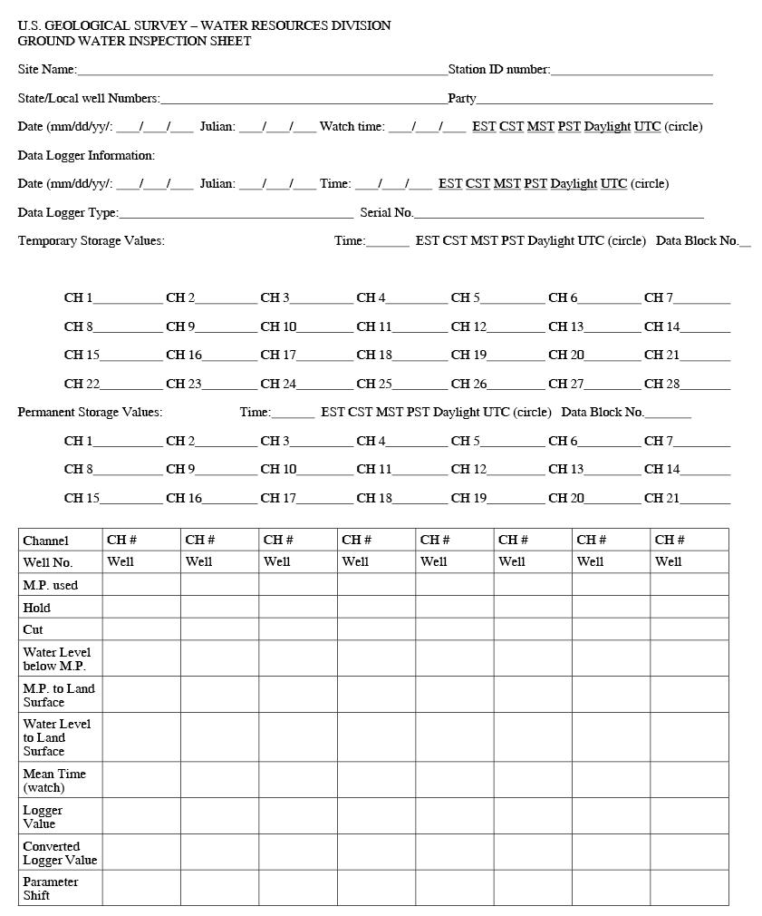
Figure 43. Ground-water inspection sheet.
The inspection form also contains a place to record the raw sensor output from the data logger, as well as the value converted to units of measurement (feet, meters). A project may have a policy of recording actual sensor output (mv, psi, ma) rather than converting the value to a measurement unit in the data logger program itself. There are several advantages to this policy when troubleshooting system problems, looking at sensor performance, and determining if the sensor is within its operating or calibration ranges. This sheet provides a place to document the sensor output; then, using the calibration equation developed for the specific transducer, document the associated converted value.
Retrieving data while in the field involves a number of steps that are performed in a certain order:
Because verifying the sensor output is crucial to determining the validity of recorded data, it must be done routinely in the field. Measure ground water levels using a steel tape or calibrated electric tape. At a minimum, verify the instrument output each time data are retrieved at the site, but verification measurements also are recommended during visits when data are not retrieved. In either case, the verification measurements should be compared with the output from the site's instrumentation at the time of the measurement. Verification measurements, commonly referred to as calibration checks, are necessary for troubleshooting, drift determination, and data correction during office computation.
Field verification measurements of ancillary data also can be useful in determining data integrity. These data might include the output of voltage from the power supply, barometric pressure, shelter temperature, and outside air temperature, all of which should be compared with the recorded values. These checks serve as an alert to a variety of potential problems and will help prevent loss of data or instrument damage.
Data may be collected in different formats. Some hydrologists prefer to collect raw data from the pressure transducer and convert the data in the office. Others prefer to collect data in a format identical to the units used during field calibration checks. Another option is to program the data logger to provide water-level elevations. Whatever the preference, maintaining a record of adjustments to the data, whether they occur in the data logger program or in the office, is essential. Data loggers can be programmed in a multitude of ways that allow project-specific or site-specific data formats.
Use a field note with a checklist of steps and measurements to record all field observations and the current data from the data logger. It provides a historical record of field activities.
Keep a log for the site in the instrument shelter. The log serves as a troubleshooting aid, as a quick historical reference to water-level trends, equipment problems, and as a long-term record of changes and occurrences at the particular site. At each site, keep a printed copy of the data logger program being used in the instrument shelter.
In the office, maintain a binder with field information similar to that recorded on the site log so that a general historical record is available there and can be referred to before and after a field trip. Other information to be included are site descriptions and road logs, transducer ratings, programming instructions, and phone numbers and addresses of important contacts.
After retrieving the recorded data in the field, the data must be processed and loaded into a data base. A recommended sequence for processing data is
The USGS requires that raw data be permanently archived prior to any alteration of the data set. Recommendations for archiving electronically recorded (and other) data are presented in Hubbard (1992) and were established as official policy by WRD Memorandum 92.59 with modifications contained in WRD Memorandum 99.33 (U.S. Geological Survey, 1992 and 1999). After the data have been loaded into the data base, they can be manipulated appropriately during the records computation process, as described below.
The first step, if necessary, is to convert pressure data to water-level data. The second step is to apply corrections obtained from field verification measurements. If the record is faulty due to instrumentation or other problems, corrections usually cannot be applied. In general, a missing or faulty record of ground-water level cannot be estimated reliably. Four types of corrections can be applied to the record—datum corrections, hung-depth corrections, drift corrections, and calibration corrections. Use time proration for the first two types of corrections. Apply a datum correction when a change has ocurred to the elevation of the measuring point of the well. Keep a level summary sheet with the site's permanent file to document reference elevation changes. A hung-depth correction can be applied if the position of the transducer changes relative to its original position, due either to purposeful or accidental raising or lowering of the transducer in the well, or to changes from other causes such as an earthquake. A drift correction—usually a linear proration with time—is applied to compensate for drift in the transducer's offset calibration. Calibration corrections can be applied either by linear time proration from the time of one calibration to the next, or by starting and ending a constant correction for a specific period of time.
The third and final step of record computation requires documenting and explaining in a station analysis how all conversion equations and other corrections were applied. The station analysis (fig. 44), written periodically after the final record is produced, should be kept with the permanent data file, along with the record computations, field notes, archival and data conversion notes, data tables, and other pertinent information.
Figure 44. Ground-water record station analysis.
Data processing requires a systematic, well-planned process fully integrated with field procedures. USGS policy for archiving data should be followed. The raw data must be corrected systematically and consistently, then documented in the station analysis that will be included with the permanent record.
Specific field applications of submersible pressure transducer and data logger systems are discussed in this section. Although submersible pressure transducers are used primarily for the collection of water-level measurements in ground water, they also can be used in surface-water and unsaturated-zone settings.
Submersible pressure transducers can be used for long-term and short-term applications. This subsection discusses both applications. A third discussion on reducing well-bore storage is presented so that the user can apply this technique to reduce the effective diameter of wells during slug tests or aquifer tests.
Many hydrologic investigations require continual monitoring (over periods of weeks to years) of water levels in wells. Examples of such studies include monitoring water levels for indication of earth tides (Galloway and Rojstaczer, 1988; Hsieh and others, 1987), indication of earthquakes (Roeloffs and others, 1989; Cooper and others, 1965), determination of temporal variation in vertical or horizontal hydraulic gradients (Garber and Koopman, 1968; Rosenberry, 1990), determination of timing and magnitude of recharge to ground water following precipitation events (Novakowski and Gillham, 1988; Rosenberry, 1990), and monitoring of pump-and-treat operations at ground-water reclamation sites. For many studies, even if continual data collection is not necessary, it is cost effective to monitor water-level fluctuations in wells with a sensor rather than using human resources to collect discrete measurements.
Submersible pressure transducers have long been used for monitoring water-level fluctuations in wells (Shuter and Johnson, 1961; Garber and Koopman, 1968). Buried in the soil, these devices also have been used for decades to monitor pressure heads. Sensors used in this application have historically been called the "Casagrande type" pressure transducer, commonly used to monitor pressure heads in and around dams. While other automated water-level sensor systems also can provide continual water-level data in wells, submersible pressure transducers are particularly well suited for some applications. Typically small, and requiring little maintenance, because they are immersed in water their environmental conditions are relatively stable. Some examples of applications in which submersible pressure transducers are particularly well suited are listed below:
As shown in the previous discussion, submersible pressure transducers are well suited for many hydrologic applications; however, their use for long-term monitoring of water levels occasionally can lead to errors if data are not corroborated. The convenience and low maintenance of submersible pressure transducers can lead to long intervals between calibration checks and overconfidence in the reliability of the sensor's data. If checks on the calibration of sensors are not made, data may be erroneous to the point of leading to incorrect hydrologic interpretations. A study of vertical hydraulic head gradients at a well nest in New Hampshire showed that uncorrected data from submersible pressure transducers resulted in an interpretation of reversals in vertical hydraulic-head gradients when none actually occurred (Rosenberry, 1990). In the New Hampshire study, linear adjustment of data based on monthly check measurements would have led to the conclusion that additional water-table fluctuations of up to 0.17 ft occurred when weekly check measurements indicated that sensor drift actually was responsible for those interpreted water-level fluctuations.
Gage pressure transducers usually are used to measure pressure in a water body open to the atmosphere, whereas absolute transducers are usually used as barometers and in sealed environments such as below packers. The user may wish to substitute absolute transducers for gage transducers to eliminate the need for vented cable, especially to multiple transducers in close proximity, connected to one data logger. A barometer, which can be an identical inexpensive absolute transducer, also must be operated. When using an absolute transducer in a gage transducer application, subtract the barometric record from the water-level record to get submergence. Three redundant barometers can be used in conjunction with many absolute transducers measuring water levels. Because the adjusted record is the difference between two records, noise and drift that are not common to both transducers may increase by as much as a factor of two.
An absolute transducer can also be used instead of a gage transducer to measure changes in wells in aquifers with barometric efficiencies close to 100 percent. After verifying that the barometric efficiency is indeed close to 100 percent, the original record from the absolute transducer is acceptable as the "barometrically adjusted" record.
Submersible pressure transducers have been used extensively for monitoring water-level fluctuations during single-well and multiple-well aquifer and slug tests. Before the use of automated sensors, aquifer tests were labor intensive, and early drawdown in the pumped well was not easily observed. Similarly, for single-well slug tests in sandy material, the early portion of the recovery commonly went unrecorded simply because it was not possible to get water-level measurements that were only seconds apart. Using submersible pressure transducers has reduced labor costs and has provided the opportunity to collect frequent data during the early portion of aquifer and slug tests. When combined with a programmable data logger, the pressure transducer can supply data frequently during the early portion of the test and, less frequently, as the test progresses and the recovery rate slows. For clean, coarse sand, when the recovery of a slug test can be completed in less than half a minute, the fast response of many types of submersible pressure transducers can allow measurement with a sampling interval of half a second or less.
The pressure transducer used for aquifer tests should be capable of reliably measuring the expected range of water-level fluctuations. For example, for an aquifer test, the pressure transducer in the pumped well should be capable of monitoring head changes much larger than is necessary for transducers installed in observation wells, where changes in water level are smaller and where greater accuracy may be desired. Similarly, for most single-well slug tests, a pressure transducer with a small pressure-sensitive range (such as 0-5 psi) is adequate.
Due to the movement of water from the well into the formation, the water level in a well or piezometer can lag behind head changes in the geologic formation. Typical situations in which this well-bore storage effect is most significant include slug tests, early time in drawdown or recovery during an aquifer test, and wells in low-permeability materials. Only in slug or bailing tests, in which a slug or water is rapidly introduced into or withdrawn from the well, is the effect of reducing well-bore storage undesirable. In fact, analyzing the decay of the residual water level in a well to determine hydraulic conductivity is the purpose of a slug test (Lohman, 1972).
Packers that seal parts of wells to prevent flow within the borehole or to isolate zones for special tests sometimes are used to minimize the effects of well-bore storage in aquifer tests. Well-bore storage is, in effect, an incremental slug test superimposed upon the water-level fluctuation of interest during the test. An inexpensive packer that can be made in the field from materials from a hardware store or lumber yard (fig. 45) encloses the transducer and seals the piezometer. The appropriate transducer for this application is an absolute device because the transducer is sealed into a zone without access to atmospheric reference through the well. Drain cleaners that expand to more than 4 in. are available; plumbing supply stores carry test seals of various kinds that can be made into packers. Straddle packers also can be assembled by using soldered copper tubing through brass fittings.
Figure 45. Drain-cleaner packer.
Small water-level differences between intervals separated by packers in a well can be measured with expensive, high-accuracy differential transducers that allow water in both ports or measured as the difference between outputs of expensive high-accuracy absolute transducers. Alternatively, low-cost differential transducers that allow water in both ports can be used. In one case, pressure differences of a fraction of an inch of water were measured between isolated intervals in a well at a submergence of more than 180 ft using a differential transducer with a full-scale range of about 10 ft of water. There was a large zero shift, but after establishing a new zero offset, valuable data were obtained at the beginning of the pumping period in spite of the fact that the pressure from submergence exceeded the overpressure specification by a factor of four and exceeded the specified range by a factor of 17.
A drop pipe that occupies much of the cross-sectional area of a well can be used to reduce storage in a well bore (fig. 46). Advantages of this design include the ability to measure the water level in the well without removing the pipe, and the ability of the well to de-gas. For wells deeper than is practical for a standpipe from the surface, the pipe can be weighted, sealed at the top, and suspended by the transducer cable or a stainless-steel cable. To prevent a change in well-bore storage with changes in water level, the pipe must extend above and below possible water-level fluctuations. The appropriate transducer for this application is a differential or vented device, because the transducer is in water open to the atmosphere.
Figure 46. Drop-pipe protection of a submerged transducer.
Submersible pressure transducers increasingly are being used for monitoring stage at surface- water gages. This is due to their ease of installation and maintenance, relatively low cost, and minimal requirements for shelter size, factors which provide more versatility in locating the instrumentation. For surface-water applications, a desirable transducer
No submersible transducer currently is satisfactory for long-term, unattended use in surface-water stage monitoring under all environmental conditions. Because of their siting versatility and their low cost for short-term surface-water studies, submersible pressure transducers will continue to be used in surface-water monitoring programs. The following basic installation guidelines and limitations are intended to assist in determining the suitability of a submersible pressure transducer for a given surface-water monitoring program.
An important consideration in planning for the use of a submersible transducer at a surface water installation is to minimize the difficulty of servicing the transducer during calibration and repair. Gaging station designs should enable one person to remove and re-install the transducer.
Two advantages of using submersible pressure transducers for monitoring surface-water stage are the minimal space requirements of the data acquisition system, and lack of the need to provide a pressurized gas-purge system and pressure tank (Lamb, 1994). This allows the use of a much smaller weatherproof enclosure to house the data logger, battery and data relay equipment. If necessary, the entire sensing and recording system can be contained in one or two small environmental enclosures. Attach the transducer cable to the data logger by passing it through a small-diameter weatherproof strain-relief fitting in the wall of the enclosure.
These small enclosures can be located in places where larger shelters needed for pressurized gas-purge systems cannot. Some types of submersible transducers can be used with data and vent tube cables that are as long as 1000 ft, thus allowing shelter placement above the reach of flood waters. Smaller shelters can just as easily be mounted on a bridge deck or railing. They can be easily installed for short-term monitoring, then moved to another location. For example, portable installations were used successfully during the 1993 mid-western floods, which allowed the USGS to continue monitoring the rise of floodwaters that had inundated original fixed gaging stations (H. Hauck, U.S. Geological Survey, oral comm., 1998). These systems also can be readily adapted to transmit data by radio or satellite.
Two types of surface-water installations can best use submersible pressure transducers to monitor the stage of streams: the first type of installation uses a transducer submerged directly in the stream at the end of a protective steel conduit (fig. 47); the second type uses a submersible transducer placed in a stilling well. Each type of installation has benefits and drawbacks. A stilling well is most desirable in terms of access for servicing, maintenance and replacement, and for damage protection during high flows and freezing. However, the operation of stilling wells is subject to the safety regulations applicable to confined spaces. A steel conduit is most desirable if the recording instruments must be located a substantial distance from the stream, either horizontally or vertically. In either use, the transducer needs to be installed securely so that it does not move relative to gage datum and so that the transducer cable is protected. As in ground-water applications, care must be taken during installation and operation that moisture or other material does not enter the gage transducer's vent tube. During installation, this can be accomplished by wrapping the end of the vent tube with waterproof tape while pulling the tube through the steel conduit. After installation, a desiccating system that includes a thin, flexible moisture barrier should be used to keep the air in the vent tube dry, yet still allow the transducer to register small changes in atmospheric pressure.
Figure 47. Surface-water monitoring installation.
When they are installed in a stilling well, submersible pressure transducers are mounted vertically. The most common type of surface-water installation, however, uses a steel conduit anchored down a sloped bank, which leaves the transducer oriented out of vertical. If the transducer is oriented out of the vertical, care must be used after servicing to reposition the transducer in precisely the same orientation. Calibration must then be checked against an independent measurement of stage. Static tubes and crest-stage-gage bottom caps can be used to eliminate velocity-head effects on the transducer (Kaehlre and Thibodeaux, 1994). A static tube, a device used to minimize the effects of turbulent flow, is a pipe with holes drilled into it at regular intervals. The transducer is secured at the end of the steel conduit, the static tube is placed over the transducer, threaded onto the end of the steel conduit, and a cap secured to the end of the static tube.
Other methods include installing transducers in a series of crest-stage gages or in a conduit with the transducer attached to a flexible handle that can be removed for easy cleaning of the transducer. Both of these methods provide a fixed resting point for the transducer at a known gage elevation.
As with any stage sensing instrument, records must be maintained to help evaluate the accuracy and reliability of transducers used in surface-water monitoring (Kirby, 1994). Field observations necessary for comparison with the output from the transducer over the range of stage recorded should include water-level readings obtained from an established reference gage; and peak stages registered by crest-stage-gages and outside high water marks. Elevations of the reference and principal gages should be verified periodically by level surveys run from established reference or bench marks using approved USGS methods (Kennedy, 1990). If necessary, use comparisons between the field observations and the recorded transducer values to adjust the data. Check and re-calibrate the transducer when field comparisons show a substantial departure from the reference or principal gage readings. Calibration and re-calibration should be done over the range that reflecting the expected range of stage. Refer to sections in this report on calibration and field calibration for specific procedures.
Instrument drift and the influence of changes in barometric pressure, temperature, and humidity on the long-term operation of transducers have been discussed earlier in this report. Another concern for long-term deployment is that transducers have, by design, a multiconductor cable connecting the transducer assembly to a data logger, which may provide a path for voltage surges from lightning strikes near the water.
Transducers and other electronic sensors placed in the water and having a common electrical connection to a data logger may cause a ground loop to form between the various sensors. If the data logger is attached to an earth ground and readings are erratic for one or more of the attached sensors, a ground loop should be suspected. A possible solution is to remove the earth ground from the data logger, but this may make the data logger more vulnerable to damage from a voltage surge.
Variable water temperature in streams can be a problem for submersible transducers. Many transducers are not temperature compensated, and those that are may not have sufficiently accurate or responsive temperature-sensing capabilities. In any case, submersible pressure transducers should not be operated where water will freeze in the port, as that will destroy most pressure transducers.
As in ground-water applications, certain types of recorded ancillary data can be very beneficial. Monitoring the changes in transducer and data logger temperature can help determine when temperatures are outside the instrument's operating limits. Because surface-water temperatures fluctuate, in contrast to ground-water temperatures (which usually stay nearly constant), it is important to monitor water temperature in surface-water data collection efforts because temperature compensation affects the transducer's performance. Recording the battery voltage of the data logger also can help ascertain the integrity of the power supply, whether it be a solar charged battery system, a battery on its own, or AC power with battery backup. Review the battery voltage data to detect power supply problems before they cause the loss of data. Also, record the barometric pressure. Absolute (non-vented) transducers must have their output compensated for barometric pressure in order to record or compute the water level elevation. Gage (vented) transducers are self-compensating as long as the inside of the vent tube remains dry and unobstructed. In the event these conditions are not met, comparison with the recorded barometric pressure can aid in determining if the data are flawed.
Figure 48. Soil-water tensiometer.
Figure 49. Field tensiometer installation.
Pore space within the unsaturated zone is occupied by either water or air. Water is held under tension (i.e., pressure is less than atmospheric) by the capillary attraction of small pores. Tensiometers are used to measure liquid water pressure under unsaturated conditions. Air pressures in the unsaturated zone, which may be greater than or less than atmospheric pressure, are measured with soil-gas piezometers. Pressure transducers can be used in conjunction with either of these devices.
Because pressure head of liquid water above the water table (hp) generally is less than atmospheric, transducers used with tensiometers must be capable of measuring negative pressure or vacuum. Tensiometers are functional when hp ranges from 0 to about -400 in. of water gage pressure. Principles of tensiometer operation and design are described in Gardner and others (1922), Cassel and Klute (1986), and Stannard (1986). A typical design is shown in figure 48. The body of the tensiometer is a PVC tube filled with water, the bottom of which contains a porous ceramic cup inserted into the soil. The ceramic cup forms a continuum with the soil pores, allowing soil-water pressures (suction) to be transmitted to the tensiometer. The top end of the tensiometer is fitted with some sort of pressure-sensing device. Original tensiometer designs used mercury or water manometers or vacuum gauges, but gage or absolute pressure transducers, allowing automatic recording, are now more commonly used (for example, Yeh and others, 1986). Tensiometers usually are installed vertically from land surface, although constructing a trench or tunnel permits horizontal installation.
Measurements of hp at a number of depths in the unsaturated zone are desirable in order to measure the magnitude of the hydraulic gradient and infer the direction of water movement. A typical field site might be equipped with 10 or more tensiometers. Switchable valve systems have been developed that scan all tensiometers with a single transducer. Yeh and others (1986) used a hypodermic needle attached to a pressure transducer to manually record several hundred tensiometer readings in a short period of time, the needle being inserted through a rubber stopper on each tensiometer. When inexpensive pressure transducers became available, it became feasible to fit each tensiometer with a separate transducer, thus avoiding complicated switching valves and allowing automatic recording.
When selecting the pressure range of a transducer, keep in mind that the pressure (P) recorded by the differential-pressure transducer will record the total head (ht) at the measurement depth of the tensiometer (Z1, for example). That is, P = ht and ht accounts both for pressure head and gravity head, ht = hp - Z1. So the pressure head at Z1 is calculated as hp = ht + Z1. If the water table were at Z1, then by definition hp would be 0 and P would equal - Z1. The appropriate pressure range for transducers depends on the specific application: a range of 0 to -400 in. of water is sufficient for most field studies, whereas a smaller range allows for more accuracy and may be desirable for laboratory experiments or detailed field studies. In selecting the pressure range, the gravity component Z1 (due to the hanging water column from the transducer to the ceramic cup) must be considered. If the anticipated range of pressure heads for a study is between 0 and -5 in., but Z1 is 20 in., then the transducer must be capable of sensing pressures in the range of -20 to -25 in. The need to account for Z1 limits the depths from land surface to which tensiometers can be installed. Some researchers avoid this limitation by burying both the transducer and the ceramic cup. In other cases trenches, tunnels, or caissons have been constructed to allow horizontal installation of tensiometers. This construction permits deeper installation and minimizes Z1 so that transducers with smaller pressure ranges can be employed.
Because the water within a tensiometer is under a vacuum, air tends to slowly come out of solution and accumulate within it. Most tensiometers are equipped with a flushing valve to permit periodic removal of that air. The inability to remove the air from buried tensiometers may severely limit their use. Systems of tensiometers with transducers should be designed to minimize accumulated air, which expands and contracts as its temperature rises and falls, causing pressure head oscillations that are correlated with temperature in the recorded data. Ideally, tensiometers and pressure transducers should be insulated and shielded from direct solar radiation. In field studies, this shielding may be accomplished by enclosing the top of the tensiometer and transducer in a container that can be buried a few inches below ground, as shown in Figure 49.
Measurements of soil-gas pressures may be made for determining barometric efficiency of geologic units (Weeks, 1978) or for monitoring of pneumatic tests (Baehr and Hult, 1991). Both operations are designed for calculating the air permeability of partially saturated porous media. Data from soil-gas piezometers constructed in the unsaturated zone are obtained by drilling a borehole and installing a small diameter tube (the diameter is usually not greater than 0.25 in.) open at the bottom and extending from the measurement point to land surface. After sealing the borehole, attach a pressure transducer to the top of the tube. Determination of barometric efficiency relies on measuring changes in barometric pressure and the time it takes for those changes to be propagated down to the piezometer, and analysis requires a barometer (an absolute-pressure transducer) in addition to the gage or absolute transducer attached to the tube. Gage transducers with a pressure range of plus and minus a few inches of water are usually preferred for measuring soil-gas pressures because they encompass the typical range in diurnal barometric fluctuations. Either absolute or gage transducers with a wider range of pressure may be used for monitoring pneumatic tests.
Submersible pressure transducers generally require minimal maintenance, but problems can arise if they are not checked periodically. The following is a list of common problems encountered by the authors, and some suggested solutions to these problems. Occasionally, a problem can be solved only by replacing the transducer, but more commonly problems can be corrected in the field.
Failure of submerged transducers commonly is caused by water leaking into the housing. Transducer leakage can appear in the data as an unexplained step or as measurements that cease, move out of range, or fluctuate wildly. Techniques to prevent leakage include the use of welded seals, O-ring seals, potted electronics and soldered contacts, sealed strain-relief fittings, and rubberized boots covering connections between the cable and the transducer's housing. Any of these components, however, can fail. Multiple layers of waterproofing, which can be user tested, can prevent leakage, failure, and lost data (fig. 50). A double housing with an intervening chamber can be left pressurized so that if leakage occurs, dry air leaks into the water. Pressurize the chamber only slightly above the anticipated water pressure to prevent rupturing the seals. The chamber with strain reliefs shown in figure 50 has been tested to a pressure of 115 ft of water. In practice, the residual air pressure sometimes decays, allowing a small amount of leakage into the chamber. The inner housing then prevents that small amount of water from penetrating to the transducer. Chambers have been used without any leakage for more than five years. During one application in which two commercial transducers failed after only one month each in service, encasing the third commercial transducer in just the inner chamber produced 14 years of troublefree data.
Figure 50. Pressurized housing for pressure transducer.
Figure 51. Housing for cable splice.
Commercial vented transducer cable must commonly be spliced. A waterproof splice can be made using strain reliefs and PVC pipe fittings (fig. 51). Connect the vent tubes with tubing of about the same diameter so that the cavity does not act as a pressure accumulator, restricting transmission of barometric pressure changes. For added security, the cable splice can be doubled in the same way as the pressurized housing shown in figure 50. Besides their primary functions of reducing well-bore storage, the drain-cleaner packer (fig. 45) and the drop pipe (fig. 46) both act as additional waterproof housings for pressure transducers. In waterproofing transducers, user experimentation and testing are essential. Providing additional waterproofing can greatly reduce the incidence of lost data.
The most frequent problems encountered when collecting water-level data with a pressure transducer and data logger include open and short circuits. An open circuit can result in data floating erratically or resting at zero or the offset value. A short commonly results in data values that indicate an over-range condition for the data logger. Solutions are to check the connections of the wires to the data logger wiring panel (where shorts most commonly occur) and to check the wire for cuts, kinks, and abrasions. Tinning leads reduces the chances of short circuits from unattached wire strands and also prevents or reduces noise. Find short circuits by testing the resistance between the drain or ground wire and each excitation and sensing lead. When resistance is not infinite, there is a short. Find open circuits by measuring the resistance across the excitation lead pair and the sensing lead pair. It should be equal to the resistance across the bridge to which the lead or excitation pair is attached, commonly about 100 ohms for metal strain-gage transducers and 1,000 to 5,000 ohms for silicon strain-gage transducers.
Excessive levels of noise in the data sometimes can be attributed to one or more loose ground wires. Securely attach ground wires to either a ground terminal on the data logger, or to a grounding rod. Take care to maintain only one ground in order to avoid problems with ground loops, which could result in considerable noise. In some applications, the pressure transducer and data logger are not grounded, in which case the installation is termed a 'floating system.' In this situation, connect ground wires only to the ground terminal on the data logger.
Failure of the pressure-transducer diaphragm commonly is caused by transmission of pressure waves through the water column, sometimes referred to as water hammer. Strong pressure waves can severely over-pressure the transducer and rupture the diaphragm, resulting in sudden loss of data. The diaphragm also can fail if the transducer is dropped onto a hard surface, or if it is rapidly dropped to the water surface while lowering the device inside a well. Water freezing in the transducer can likewise rupture the diaphragm. Diaphragm failure requires replacing the transducer.
An interruption of the power supply to most submersible pressure transducers will result in the output changing to zero or to the offset value entered into the data logger. The solution is to resupply power to the transducer. Commonly, if power to the data logger is lost, data already collected and stored in random access memory (RAM) in the data logger are lost. No additional data will be collected until power is restored and the data-collection program is reentered. A partial remedy is to install a backup data-storage device, or use a data logger with a nonvolatile memory, to retain data already recorded as well as the data logger program. A charging system (solar or AC trickle) can help prevent power loss.
The internal circuitry in the data logger fails infrequently. However, this problem is difficult to diagnose because an open circuit in the wiring between the data logger and the transducer can have the same effect on the data. If a channel in the data logger fails, output values drift erratically. Occasionally, the data logger averages this erratic drift to a value similar to the expected value, making the failure difficult to notice. One solution is to reconnect the sensor to a different, but still functioning, channel on the data logger; another is to replace the data logger. Occasionally the problem is created by contaminants (such as oil, water, or perspiration) that create shorts between data logger channels, in which case a solution is to disassemble and clean the wiring panel on the data logger.
The data logger's wiring panel also can become corroded after extended operation in humid conditions. Corrosion can cause an intermittent open circuit between the wire and the wiring panel, causing intermittent periods of erroneous data. The solution requires cleaning the connections, and changing the environment in which the data logger is housed. Operation in a drier environment (for example, enclosing the data logger in a low-humidity container or frequently replacing the desiccant) prevents corrosion-related problems. Fumes released from a battery enclosed in the data logger's housing also can cause corrosion. To avoid this problem, house the battery in a separate location from the data logger.
Voltage surges (transients) can cause a multitude of problems, ranging from alteration of the data logger program or alteration of the data logger clock, to complete failure of the data logger and pressure transducer. A transient current from a nearby lightning strike can corrupt data without harming either the data logger or the pressure transducer. One solution is to turn off the data logger, resupply power, and then reenter the program, but proper grounding will solve most problems associated with transient voltage surges. A direct lightning strike, however, will probably destroy both data logger and the pressure transducer. Voltage surges coming through AC power lines or telephone lines can damage or destroy the transducer, the data logger and other connected electronic equipment. Surge protection devices usually are placed between these incoming lines and the data logger, but they are not normally used between the transducer and the data logger.
Faulty shielding can allow electromagnetic coupling to corrupt the signal from the sensor to the data logger. Occasionally this is caused by cuts or kinks in the transducer cable, but more frequently by long, exposed, unshielded wire near the data logger. These long wires increase the signal noise sent to the data logger. One solution is to minimize the length of unshielded wire. A second solution is to change the program in the data logger to increase the signal or the excitation from the data logger, effectively increasing the signal-to-noise ratio. A third solution is to increase signal integration time during the measurement cycle.
An over-range problem develops when the signal is increased beyond the anticipated maximum value. Many data loggers can be programmed to accept different ranges of sensor output. Sensor output rising beyond the anticipated maximum output programmed into the data logger creates an over-range situation. Over-range problems also can occur from submerging the pressure transducer too deeply (overpressuring), so that the transducer is subjected to pressures exceeding its maximum. Even if the pressure transducer is situated correctly, unexpected extreme water-level rises can exceed the anticipated maximum value.
Occasionally data loggers are not capable of measuring the entire voltage range that a transducer can output, thereby reducing the range of water-level measurements that can be sensed. Possible solutions are to reprogram the data logger to accept a wider range of output from the transducer, or to program the data logger to simultaneously log output from the transducer on multiple input ranges during the same measurement scan. The latter solution retains resolution while increasing the range of input signal.
Solutions to overpressure problems are to raise the pressure transducer, or use a different model of transducer capable of measuring a wider range of pressure fluctuations. In some cases, it may be possible to continue operating the transducer as long as the overpressure is not too extreme. When using this solution, the investigator should extend the calibration range to include these over-pressure conditions.
Aronson, Milton H., 1976, Low-level measurements, Part 1 — Noise: Pittsburgh, Pa., Measurements and Data Corporation, 16 p.
Aronson, Milton H., 1976, Low-level measurements, Part 2 — Magnetic Shielding: Pittsburgh, Pa., Measurements and Data Corporation, 16 p.
Aronson, Milton H., 1976, Low-level measurements, Part 3 — Electrostatic Shielding: Pittsburgh, Pa., Measurements and Data Corporation, 16 p.
Aronson, Milton H., Low-level measurements, Part 4 — Shields and Ground Loops: Pittsburgh, Pa., Measurements and Data Corporation, 16 p.
Baehr, A.L., and Hult, M.F., 1991, Evaluation of unsaturated zone air permeability through pneumatic tests: Water Resources Research, Vol 27, no. 10, pp 2605–2617.
Bell & Howell, 1983, Pressure transducer handbook: Pasadena, Calif., Division of CEC Instruments, 143 p.
Benedict, Robert P., 1984, Fundamentals of temperature, pressure, and flow measurements: New York, John Wiley and Sons, 532 p.
Boucher, Michelle S., 1994, Precision and accuracy of manual water-level measurements taken in the Yucca Mountain area, Nye County, Nevada: U.S. Geological Survey Water-Resources Investigations WRI 93-4025, 18p.
Carpenter, M.C., 1994, High-accuracy measurements with inexpensive pressure sensors— assembly, calibration, and use; in Hollett, K.J., Wilbourn, S.L., and Latkovich, V.J., compilers, Proceedings of a U.S. Geological Survey Workshop on the Application and Needs of Submersible Pressure Sensors, Denver, Colorado, June 7–10, 1994: U.S. Geological Survey Open-File Report 94-531, p.5–9.
Carpenter, M.C., Carruth, R.L., Fink, J.B., Boling, J.K., and Cluer, B.L., 1995, Hydrogeology and deformation of sandbars in response to fluctuations in flow of the Colorado River in the Grand Canyon, Arizona: U.S. Geological Survey Water-Resources Investigations Report 95–4010, 16 p.
Carpenter, M.C., Hanson, R.T., and Riley, F.S., 1987, An averaging temperature sensor to correct measurements of aquifer compaction for interaquifer borehole flow: American Geophysical Union Transactions, v. 68, no. 44, p. 1300.
Cassel, D.K., and Klute, Arnold, 1986, Water potential: tensiometry, in Klute, Arnold, ed. Methods of Soil Analysis: Part 1—Physical and Mineralogical Methods, American Society of Agronomy, Madison, WI, 1188 p.
CEC Instruments, no date, Pressure Transducer Handbook: Pasadena, Calif., CEC Instruments, 150 p.
Cooper Jr., H.H., Bredehoeft, J.D., Papadopulos, I.S., and Bennett, R.R., 1965, The response of well-aquifer systems to seismic waves: Journal of Geophysical Research, v. 70, no. 16, p. 3915–3926.
Data Instruments, Inc., 1981, Pressure Transducer Applications: Lexington, Mass., Data Instruments, Inc., 40p.
Freeman, L.A., 1996, Time-series ground-water-level and aquifer-system compaction data, Edwards Air Force Base, Antelope Valley, California, January 1991 through September 1993: U.S. Geological Survey Open-File Report 96–186, 32 p.
Galloway, D. and Rojstaczer, S., 1988, Analysis of the frequency response of water levels in wells to earth tides and atmospheric loading, in Hitchon B. and Bachu, S, eds., Proceedings—Fourth Canadian/American Conference on Hydrogeology, Fluid Flow, Heat Transfer and Mass Transport in Fractured Rocks, Banff, Alberta, Canada, June 21–24, 1988, p. 100–113.
Garber, M.S., and Koopman, F.C., 1968, Methods of measuring water levels in deep wells: U.S. Geological Survey Techniques of Water-Resources Investigations, Book 8, chap. A1, 23 p.
Gardner, W., Israelsen, O.W., Edlefsen, N.E., and Clyde, D., 1922, The capillary potential function and its relation to irrigation practice: Physical Review, v. 20, p. 196.
Gould, Inc., 1966, Introduction to transducers for instrumentation: Oxnard, Calif., Measurements Systems Division, 61 p.
Gillum, D.R., 1982, Industrial pressure measurement: Research Triangle Park, N.C., Instrument Society of America, 107 p.Healy, R. W., deVries, M. P., and Striegl, R. G., 1986, Concepts and data-collection techniques used in a study of the unsaturated zone at a low-level radioactive waste disposal site near Sheffield, Illinois: U.S. Geological Survey Open-File Report 85-4228, 37p.
Hollett, K.J., Wilbourn, S.L., Latkovich, V.J., 1994, Proceedings of a U.S. Geological Survey Workshop on the application and needs of submersible pressure sensors, Denver, Colorado, June 7–10, 1994: U.S. Geological Survey Open-File Report 94-531, 53 p.
Hsieh, P.A., 1993, Some experience gained from using packers and transducers in ground-water investigations of crystalline-rock aquifers, in Latkovich, V.J., ed., 1993, Proceedings of a pressure transducer-packer workshop, June 25–28, 1991: U.S. Geological Survey Open-File Report 93-71, p. 5–7.
Hsieh, P.A., Bredehoeft, J.D., and Farr, J.M., 1987, Determination of aquifer transmissivity from earth tide analysis: Water Resources Research, v. 23, no. 10, p. 1824–1832.
Hubbard, E.F., comp., 1992, Policy recommendations for management and retention of hydrologic data of the U.S. Geological Survey: U.S. Geological Survey Open-File Report 92-56, 32 p.
Instrument Society of America, 1970, Specifications and tests for strain gage pressure transducers: Pittsburgh, Pa., Instrument Society of America, S37.3.
Jones, J.C., Tracey, D.C., Sorenson, F.W., 1991, Operating manual for the U.S. Geological Survey's data-collection system with the Geostationary Operational Environmental Satellite: U.S. Geological Survey Open-File Report 91-99, 237 p.
Kaehrle, W.R, and Thibodeaux, K.G., 1994, Testing of submersible pressure transducers installed in crest-stage gage pipes; in Proceedings of a U.S. Geological Survey Pressure-Sensor Workshop, Denver, Colorado, July 28–31, 1992: U.S. Geological Survey Open-File Report 94-363, 53 p.
Keithley Instruments, Inc., 1992, Low level measurements: Cleveland, Ohio, Keithley Instruments, Inc. 172 p.
Kennedy, E.J., 1990, Levels at streamflow gaging stations: U.S. Geological Survey Techniques of Water-Resources Investigations, book 3, chap. A19, 31 p.
Kirby, W.H., 1994, Analysis of errors in stage measurements by pressure sensors, in Proceedings of a U.S. Geological Survey Pressure-Sensor Workshop, Denver, Colorado, July 28-31, 1992: U.S. Geological Survey Open-File Report 94-363, 53 p.
Lamb, T.E., 1994, History of use of submersible and nonsubmersible transducers in Arkansas, in Proceedings of a U.S. Geological Survey Pressure-Sensor Workshop, Denver, Colorado, July 28–31, 1992: U.S. Geological Survey Open-File Report 94-363, 53 p.
Lohman, S.W., 1972, Ground-Water Hydraulics, U.S. Geological Survey Prof. Paper 708, 70 p.
Lovell, A.D., Ellis, J.W., Brice, R.R., and Thomas, A.W., 1978, Remote sensing of water levels in small-diameter wells: Agricultural Engineering, v. 59, no. 10, p. 44–45.
Measurements and Data Corporation, 1986, Pressure measurement, Part 1 — Units, Standards & Part 2 — Transducers: Pittsburgh, Pa., 32 p.
Meyers, N.C., 1994, Possible designs and installation of submersible pressure transducers for use during floods, in Proceedings of a U.S. Geological Survey Workshop on the Application of Submersible Pressure Sensors, Denver, Colorado, June 7–10, 1994: U.S. Geological Survey Open-File Report 94-531, 53 p.
Novakowski, K.S., and Gillham, R.W., 1988, Field investigations of the nature of water-table response to precipitation in shallow water-table environments: Journal of Hydrology, v. 97, no. 1-2, p. 23–32.
O'Brien, G.M., 1993, Monitoring static water levels in the Yucca Mountain area, in Latkovich, V.J., ed., 1993, Proceedings of a pressure transducer-packer workshop, June 25–28, 1991: U.S. Geological Survey Open-File Report 93-71, p. 31–32.
Robson, S.G., 1993, Use of packers and transducers in aquifer tests in Castle Pines, Colorado, in Latkovich, V.J., ed., 1993, Proceedings of a pressure transducer-packer workshop, June 25–28, 1991: U.S. Geological Survey Open-File Report 93-71, p. 25.
Roeloffs, E.A., Burford, S.S., Riley, F.S. and Records, A.W., 1989, Hydrologic effects on water level changes associated with episodic fault creep near Parkfield, California: Journal of Geophysical Research, v. 94, no. B9, pp. 12387–12402.
Rosenberry, D.O., 1990, Effect of sensor error on interpretation of long-term water-level data: Groundwater, v. 28 no. 6, pp. 927–936.
Schaefer, M.E., and Hemond, H.F., 1986, A low-cost system to remotely measure piezometric head: Ground Water Monitoring Review, v. 6, no. 2, pp. 87–91.
Shuter, E. and Johnson, A.I, 1961, Evaluation of equipment for measurement of water level in wells of small diameter: U.S. Geological Survey Circular 453, 12 p.
Stannard, D.I., 1986, Theory, construction and operation of simple tensiometers: Ground Water Monitoring Review, Vol. 6, no. 3, pp 70–78.
Taylor, C.J. and Alley, W.M., 2001, Ground-water level monitoring and the importance of long-term water-level data, U.S. Geological Survey Circular 1217, 68 p.
U.S. Geological Survey, 1992, Policy for management and retention of hydrologic data of the U.S. Geological Survey: U.S. Geological Survey Water Resources Division Memorandum 92.59, accessed March 25, 1999, at URLhttp://water.usgs.gov/admin/memo/WRD/wrdpolicy99.33.html
Van Doren, Tom, 1991, Grounding and shielding electronic systems: Rolla, Missouri, University of Missouri, 160 p.
Weeks, E.P., 1978, Field determination of vertical permeability to air in the unsaturated zone: U.S. Geological Survey Prof. Paper 1051, 41p.
Yeh, T-C., J., Gelhar, L.W., and Wierenge, P.J., 1986, Observations of spatial variability of soil-water pressure in a field soil: Soil Science, v. 142, no. 1, pp. 7–12.
The U.S. Geological Survey publishes a series of manuals describing procedures for planning and conducting specialized work in water-resources investigations. The material is grouped under major subject headings called books and is further divided into sections and chapters. For example, Section A of Book 3 (Applications of Hydraulics) pertains to surface water. The chapter, the unit of publication, is limited to a narrow field of subject matter. This format permits flexibility in revision and publication as the need arises.
The reports listed below are for sale by the U.S. Geological Survey, Branch of Information Services, Box 25286, Federal Center, Denver, Colorado 80225 (authorized agent of the Superintendent of Documents, Government Printing Office). Prepayment is required. Remittance should be sent by check or money order payable to the U.S. Geological Survey. Prices are not included because they are subject to change. Current prices can be obtained by contacting the Branch of Information Services (ph: (303) 202-4700; fax: (303) 202-4693; e-mail: infoservices@usgs.gov). When ordering or inquiring about prices for any of these publications, please give the title, book number, chapter number, and "U.S. Geological Survey Techniques of Water-Resources Investigations."
A current list of Techniques of Water-Resources Investigations is available on the World Wide Web at the following URL: http://water.usgs.gov/lookup/get?twri.
1-D1. Water temperature – influential factors, field measurement, and data presentation, by H.H. Stevens, Jr., J.F. Ficke, and G.F. Smoot: USGS – TWRI Book 1, Chapter D1. 65 pages. 1975.
1-D2. Guidelines for collection and field analysis of ground-water samples for selected unstable constituents, by W.W. Wood: USGS – TWRI Book 1, Chapter D2. 24 pages. 1976.
2-D1. Application of surface geophysics to ground-water investigations, by A.A.R. Zohdy, G.P. Eaton, and D.R. Mabey: USGS – TWRI Book 2, Chapter D1.116 pages. 1974.
2-D2. Application of seismic-refraction techniques to hydrologic studies, by F.P. Haeni: USGS – TWRI Book 2, Chapter D2. 86 pages. 1988.
2-E1. Application of borehole geophysics to water-resources investigations, by W.S. Keys and L.M. MacCary: USGS – TWRI Book 2, Chapter E1. 126 pages. 1971.
2-E2. Borehole geophysics applied to ground-water investigations, by W.S. Keys: USGS – TWRI Book 2, Chapter E2. 150 pages. 1990.
2-F1. Application of drilling, coring, and sampling techniques to test holes and wells, by Eugene Shuter and W.E. Teasdale: USGS – TWRI Book 2, Chapter F1. 97 pages. 1989.
3-A1. General field and office procedures for indirect discharge measurements, by M.A. Benson and Tate Dalrymple: USGS – TWRI Book 3, Chapter A1. 30 pages. 1967.
3-A2. Measurement of peak discharge by the slope-area method, by Tate Dalrymple and M.A. Benson: USGS – TWRI Book 3, Chapter A2. 12 pages. 1967.
3-A3. Measurement of peak discharge at culverts by indirect methods, by G.L. Bodhaine: USGS – TWRI Book 3, Chapter A3. 60 pages. 1968.
3-A4. Measurement of peak discharge at width contractions by indirect methods, by H.F. Matthai: USGS-TWRI Book 3, Chapter A4. 44 pages. 1967.
3-A5. Measurement of peak discharge at dams by indirect methods, by Harry Hulsing: USGS – TWRI Book 3. Chapter A5. 29 pages. 1967.
3-A6. General procedure for gaging streams, by R.W. Carter and Jacob Davidian: USGS – TWRI Book 3, Chapter A6. 13 pages. 1968.
3-A7. Stage measurement at gaging stations, by T.J. Buchanan and W.P. Somers: USGS – TWRI Book 3, Chapter A7. 28 pages. 1968.
3-A8. Discharge measurements at gaging stations, by T.J. Buchanan and W.P. Somers: USGS – TWRI Book 3, Chapter A8. 65 pages. 1969.
3-A9. Measurement of time of travel in streams by dye tracing, by F.A. Kilpatrick and J.F. Wilson, Jr.: USGS – TWRI Book 3, Chapter A9. 27 pages. 1989.
3-A10. Discharge ratings at gaging stations, by E.J. Kennedy: USGS – TWRI Book 3, Chapter A10. 59 pages. 1984.
3-A11. Measurement of discharge by the moving-boat method, by G.F. Smoot and C.E. Novak: USGS – TWRI Book 3, Chapter A11.22 pages. 1969.
3-A12. Fluorometric procedures for dye tracing, Revised, by J.F. Wilson, Jr., E.D. Cobb, and F.A. Kilpatrick: USGS- -TWRI Book 3, Chapter A12. 34 pages. 1986.
3-A13. Computation of continuous records of streamflow, by E.J. Kennedy: USGS – TWRI Book 3, Chapter A13. 53 pages. 1983.
3-A14. Use of flumes in measuring discharge, by F.A. Kilpatrick and V.R. Schneider: USGS – TWRI Book 3, Chapter A14. 46 pages. 1983.
3-A15. Computation of water-surface profiles in open channels, by Jacob Davidian: USGS – TWRI Book 3, Chapter A15. 48 pages. 1984.
3-A16. Measurement of discharge using tracers, by F.A. Kilpatrick and E.D. Cobb: USGS – TWRI Book 3, Chapter A16. 52 pages. 1985.
3-A17. Acoustic velocity meter systems, by Antonius Laenen: USGS – TWRI Book 3, Chapter A17. 38 pages. 1985.
3-A18. Determination of stream reaeration coefficients by use of tracers, by F.A. Kilpatrick, R.E. Rathbun, Nobuhiro Yotsukura, G.W. Parker, and L.L. DeLong: USGS – TWRI Book 3, Chapter A18. 52 pages. 1989.
3-A19. Levels at streamflow gaging stations, by E.J. Kennedy: USGS – TWRI Book 3, Chapter A19. 31 pages. 1990.
3-A20. Simulation of soluable waste transport and buildup in surface waters using tracers, by F.A. Kilpatrick: USGS – TWRI Book 3, Chapter A20. 38 pages. 1993.
3-A21. Stream-gaging cableways, by C. Russell Wagner: USGS – TWRI Book 3, Chapter A21. 56 pages. 1995.
3-B1. Aquifer-test design, observation, and data analysis, by R.W. Stallman: USGS – TWRI Book 3, Chapter B1. 26 pages. 1971.
3-B2. Introduction to ground-water hydraulics, a programed text for self-instruction, by G.D. Bennett: USGS – TWRI Book 3, Chapter B2. 172 pages. 1976.
3-B3. Type curves for selected problems of flow to wells in confined aquifers, by J.E. Reed: USGS – TWRI Book 3, Chapter B3. 106 pages. 1980.
3-B4. Regression modeling of ground-water flow, by R.L. Cooley and R.L. Naff: USGS – TWRI Book 3, Chapter B4. 232 pages. 1990.
3-B4. Supplement 1. Regression modeling of ground-water flow – Modifications to the computer code for nonlinear regression solution of steady-state ground-water flow problems, by R.L. Cooley: USGS – TWRI Book 3, Chapter B4. 8 pages. 1993.
3-B5. Definition of boundary and initial conditions in the analysis of saturated ground-water flow systems – An introduction, by O.L. Franke, T.E. Reilly, and G.D. Bennett: USGS – TWRI Book 3, Chapter B5. 15 pages. 1987.
3-B6. The principle of superposition and its application in ground-water hydraulics, by T.E. Reilly, O.L. Franke, and G. D. Bennett: USGS – TWRI Book 3, Chapter B6. 28 pages. 1987.
3-B7. Analytical solutions for one-, two-, and three-dimensional solute transport in ground-water systems with uniform flow, by E.J. Wexler: USGS – TWRI Book 3, Chapter B7. 190 pages. 1992.
3-C1. Fluvial sediment concepts, by H.P. Guy: USGS – TWRI Book 3, Chapter C1. 55 pages. 1970.
3-C2. Field methods for measurement of fluvial sediment, by H.P. Guy and V.W. Norman: USGS – TWRI Book 3, Chapter C2. 59 pages. 1970.
3-C3. Computation of fluvial-sediment discharge, by George Porterfield: USGS – TWRI Book 3, Chapter C3. 66 pages. 1972.
4-A1. Some statistical tools in hydrology, by H.C. Riggs: USGS – TWRI Book 4, Chapter A1. 39 pages. 1968.
4-A2. Frequency curves, by H.C. Riggs: USGS – TWRI Book 4, Chapter A2. 15 pages. 1968.
4-B1. Low-flow investigations, by H.C. Riggs: USGS – TWRI Book 4, Chapter B1. 18 pages. 1972.
4-B2. Storage analyses for water supply, by H.C. Riggs and C.H. Hardison: USGS – TWRI Book 4, Chapter B2. 20 pages. 1973.
4-B3. Regional analyses of streamflow characteristics, by H.C. Riggs: USGS – TWRI Book 4, Chapter B3. 15 pages. 1973.
4-D1. Computation of rate and volume of stream depletion by wells, by C.T. Jenkins: USGS – TWRI Book 4, Chapter D1. 17 pages. 1970.
5-A1. Methods for determination of inorganic substances in water and fluvial sediments, by M. J. Fishman and L.C. Friedman, editors: USGS – TWRI Book 5, Chapter A1. 545 pages. 1989.
5-A2. Determination of minor elements in water by emission spectroscopy, by P.R. Barnett and E.C. Mallory, Jr.: USGS – TWRI Book 5, Chapter A2. 31 pages. 1971.
5-A3. Methods for the determination of organic substances in water and fluvial sediments, edited by R.L. Wershaw, M.J. Fishman, R.R. Grabbe, and L.E. Lowe: USGS – TWRI Book 5, Chapter A3. 80 pages. 1987.
5-A4. Methods for collection and analysis of aquatic biological and microbiological samples, by L.J. Britton and P.E. Greeson, editors: USGS – TWRI Book 5, Chapter A4. 363 pages. 1989.
5-A5. Methods for determination of radioactive substances in water and fluvial sediments, by L.L. Thatcher, V.J. Janzer, and K.W. Edwards: USGS – TWRI Book 5, Chapter A5. 95 pages. 1977.
5-A6. Quality assurance practices for the chemical and biological analyses of water and fluvial sediments, by L.C. Friedman and D.E. Erdmann: USGS – TWRI Book 5, Chapter A6. 181 pages. 1982.
5-C1. Laboratory theory and methods for sediment analysis, by H.P. Guy: USGS – TWRI Book 5, Chapter C1. 58 pages. 1969.
6-A1. A modular three-dimensional finite-difference ground-water flow model, by M.G. McDonald and A.W. Harbaugh: USGS – TWRI Book 6, Chapter A1. 586 pages. 1988.
6-A2. Documentation of a computer program to simulate aquifer-system compaction using the modular finite- difference ground-water flow model, by S.A. Leake and D.E. Prudic: USGS – TWRI Book 6, Chapter A2. 68 pages. 1991.
6-A3. A modular finite-element model (MODFE) for areal and axisymmetric ground-water-flow problems, Part 1: Model Description and User's Manual, by L.J. Torak: USGS – TWRI Book 6, Chapter A3. 136 pages. 1993.
6-A4. A modular finite-element model (MODFE) for areal and axisymmetric ground-water-flow problems, Part 2: Derivation of finite-element equations and comparisons with analytical solutions, by R.L. Cooley: USGS – TWRI Book 6, Chapter A4. 108 pages. 1992.
6-A5. A modular finite-element model (MODFE) for areal and axisymmetric ground-water-flow problems, Part 3: Design philosophy and programming details, by L.J. Torak: USGS – TWRI Book 6, Chapter A5, 243 pages. 1993.
6-A6. A coupled surface-water and ground-water flow model (MODBRANCH) for simulation of stream-aquifer interaction, by E.D. Swain and E.J. Wexler: USGS – TWRI Book 6, Chapter A6, 125 pages. 1996.
7-C1. Finite difference model for aquifer simulation in two dimensions with results of numerical experiments, by P.C. Trescott, G.F. Pinder, and S.P. Larson: USGS – TWRI Book 7, Chapter C1. 116 pages. 1976.
7-C2. Computer model of two-dimensional solute transport and dispersion in ground water, by L.F. Konikow and J.D. Bredehoeft: USGS – TWRI Book 7, Chapter C2. 90 pages. 1978.
7-C3. A model for simulation of flow in singular and interconnected channels, by R.W. Schaffranek, R.A. Baltzer, and D.E. Goldberg: USGS – TWRI Book 7, Chapter C3. 110 pages. 1981.
8-A1. Methods of measuring water levels in deep wells, by M.S. Garber and F.C. Koopman: USGS – TWRI Book 8, Chapter A1. 23 pages. 1968.
8-A2. Installation and service manual for U.S. Geological Survey manometers, by J.D. Craig: USGS – TWRI Book 8, Chapter A2. 57 pages. 1983.
8-B2. Calibration and maintenance of vertical-axis type current meters, by G.F. Smoot and C.E. Novak: USGS – TWRI Book 8, Chapter B2. 15 pages. 1968.
9-A1. Preparations for water sampling, by F.D. Wilde, D.B. Radtke, Jacob Gibs, and R.T. Iwatsubo: USGS – TWRI Book 9, Chapter A1, [variously paged]. 1999.
9-A2. Selection of equipment for water sampling, edited by F.D. Wilde, D.B. Radtke, Jacob Gibs, and R.T. Iwatsubo – TWRI Book 9, Chapter A2, [variously paged]. 1999.
9-A3. Cleaning of equipment for water sampling, edited by F.D. Wilde, D.B. Radtke, Jacob Gibs, and R.T. Iwatsubo – TWRI Book 9, Chapter A3, [variously paged]. 1999.
9-A5. Processing of water samples, edited by F.D. Wilde, D.B. Radtke, Jacob Gibs, and R.T. Iwatsubo – TWRI Book 9, Chapter A5, 128 pages, 1999.
9-A6. Field measurements, edited by F.D. Wilde and D.B. Radtke: USGS – TWRI Book 9, Chapter A6, [variously paged]. 1998.
9-A7. Biological indicators, edited by D.N. Myers and F.D. Wilde: USGS – TWRI Book 9, Chapter A7, [variously paged]. 1997.
9-A8. Bottom-material samples, by D.B. Radtke: USGS – TWRI Book 9, Chapter A8, [variously paged]. 1998.
9-A9. Safety in field activities, by S.L. Lane and R.G. Fay: USGS – TWRI Book 9, Chapter A9, [variously paged]. 1998.
Document Accessibility: Adobe Systems Incorporated has information about PDFs and the visually impaired. This information provides tools to help make PDF files accessible. These tools convert Adobe PDF documents into HTML or ASCII text, which then can be read by a number of common screen-reading programs that synthesize text as audible speech. In addition, an accessible version of Acrobat Reader 6.0, which contains support for screen readers, is available. These tools and the accessible reader may be obtained free from Adobe at Adobe Access.