National Water-Quality Assessment (NAWQA) Program
The mission of the U.S. Geological Survey (USGS) is to assess the quantity and quality of the earth resources of the Nation and to provide information that will assist resource managers and policymakers at Federal, State, and local levels in making sound decisions. Assessment of water-quality conditions and trends is an important part of this overall mission.
One of the greatest challenges faced by water-resources scientists is acquiring reliable information that will guide the use and protection of the Nation's water resources. That challenge is being addressed by Federal, State, interstate, and local water-resource agencies and by many academic institutions. These organizations are collecting water-quality data for a host of purposes that include: compliance with permits and water-supply standards; development of remediation plans for specific contamination problems; operational decisions on industrial, wastewater, or water-supply facilities; and research on factors that affect water quality. An additional need for water-quality information is to provide a basis on which regional- and national-level policy decisions can be based. Wise decisions must be based on sound information. As a society we need to know whether certain types of water-quality problems are isolated or ubiquitous, whether there are significant differences in conditions among regions, whether the conditions are changing over time, and why these conditions change from place to place and over time. The information can be used to help determine the efficacy of existing water-quality policies and to help analysts determine the need for and likely consequences of new policies.
To address these needs, the U.S. Congress appropriated funds in 1986 for the USGS to begin a pilot program in seven project areas to develop and refine the National Water-Quality Assessment (NAWQA) Program. In 1991, the USGS began full implementation of the program. The NAWQA Program builds upon an existing base of water-quality studies of the USGS, as well as those of other Federal, State, and local agencies. The objectives of the NAWQA Program are to:
This information will help support the development and evaluation of management, regulatory, and monitoring decisions by other Federal, State, and local agencies to protect, use, and enhance water resources.
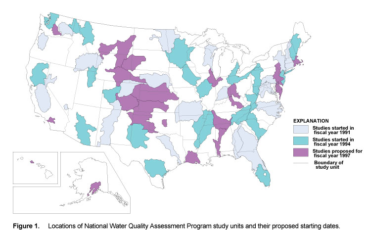
The goals of the NAWQA Program are being achieved through ongoing and proposed investigations of 60 of the Nation's most important river basins and aquifer systems, which are referred to as study units. These study units are distributed throughout the Nation and cover a diversity of hydrogeologic settings. More than two-thirds of the Nation's freshwater use occurs within the 60 study units and more than two-thirds of the people served by public water-supply systems live within their boundaries.
National synthesis of data analysis, based on aggregation of comparable information obtained from the study units, is a major component of the program. This effort focuses on selected water-quality topics using nationally consistent information. Comparative studies will explain differences and similarities in observed water-quality conditions among study areas and will identify changes and trends and their causes. The first topics addressed by the national synthesis are pesticides, nutrients, volatile organic compounds, and aquatic biology. Discussions on these and other water-quality topics will be published in periodic summaries of the quality of the Nation's ground and surface water as the information becomes available.
This report is an element of the comprehensive body of information developed as part of the NAWQA Program. The program depends heavily on the advice, cooperation, and information from many Federal, State, interstate, Tribal, and local agencies and the public. The assistance and suggestions of all are greatly appreciated.
Robert M. HirschThe National Water-Quality Assessment (NAWQA) Program was begun by the U.S. Geological Survey in 1991 as a systematic assessment of the quality of the Nation's water resources. The program will describe the status and trends in the quality of a large, representative part of the Nation's surface-water and ground-water resources and will define the primary natural and human factors affecting the quality of these resources. In meeting these goals, NAWQA will produce information that will be useful to policy makers, managers, and the general public at the national, state, and local levels. The building blocks of the NAWQA program are 60 study-unit investigations that include parts of most of the Nation's major river basins and aquifers (fig. 1). Leahy and others (1990) discuss the design of the NAWQA Program in more detail.
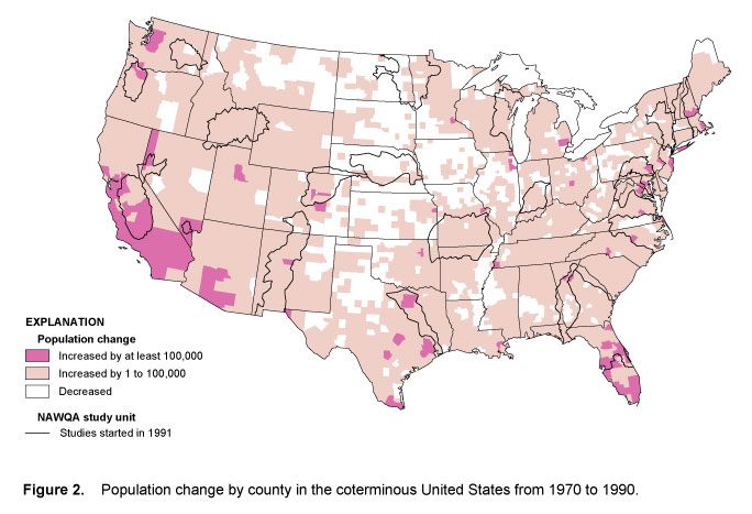
Characteristics for each of the 60 study units are being incorporated into an overall "environmental framework." This framework consists of the common natural and human factors at work across the Nation to influence water quality and provides the basis for comparing and contrasting findings across study-unit boundaries. For example, figure 2 shows population change from 1970 to 1990 by county. Study units where counties are increasing in population, such as those in California and Florida, are areas where increased urbanization and its corresponding effects on water quality could be expected.
An integrating concept for the human factors affecting water quality can be called "land use." Land use is perhaps the most important representation of the human element of the environmental framework. Certain types of land use are associated with certain human activities that affect water quality and can indicate the likely types and degree of human influence on water quality. For example, land use defined as "cropland" could be associated with specific activities, such as the application of pesticides and fertilizers, which might move into surface or ground water. Land use defined as "industrial" could be associated with the use or disposal of toxic chemicals, which also could wind up in streams or aquifers.
A nationally consistent, up-to-date (1990's timeframe), land-use data base with the resolution and detail required for NAWQA's environmental framework is not available. Data that do exist at state and local levels are not appropriate for national applications because the classification schemes are not uniform, data for whole study units sometimes do not exist, and often the data are not available in digital format. Our strategy to fill the requirement for up-to-date land use is to take the U.S. Geological Survey's generalized national georeferenced data base on land use available from the 1970's and enhance it with current, more detailed ancillary information on cropping practices and population from the 1987 Census of Agriculture and the 1990 Census of Population, respectively. In this way, numerical gradients of agricultural and urban intensities can be used to evaluate the differences between study units in agricultural and urban/suburban water-quality conditions. This approach for characterizing land use is nationally consistent and comparable, is current and detailed enough to support at least part of NAWQA's needs, relies on available data that can be used in an automated geographic information system (ARC/INFO)(1), and is realistic to achieve.
(1) Use of trade names in this report is for identification purposes only and does not constitute endorsement by the U.S. Geological Survey.This paper describes a method used to update residential land use using the 1990 Census of Population so that the extent of urban development within NAWQA study units can be compared and contrasted. The procedure uses available national data bases of land use and population, which are overlaid using the capabilities of the automated geographic system. The maps produced using this procedure illustrate where urbanization has occurred over the last 20 years (fig. 3).

The NAWQA Program needs a nationally consistent definition of a broad category of "urban" land use to document where urban land currently exists (1990) and where urbanization has occurred over the past 20 years, especially where agricultural or forest uses have changed to urban uses. Under the land-use classification system set forth by Anderson and others (1976), urban or built-up land is defined as "areas of intensive use with much of the land covered by structures." This includes subcategories for residential, commercial, industrial, and transportation uses. The procedure attempts to use population data to refine only the "residential" subcategory of urban land use, which is the component of urban land use that increased the most (50 percent) during the 1970's, according to Vesterby and others (1994).
Residential land uses range from high-density multiple-unit structures, such as apartment buildings, to low-density single-family houses on large lots typical of suburbia. In residential areas, septic tanks, sewage disposal systems, runoff from driveways and parking lots, and fertilizers and pesticides applied for lawn care can affect water quality. Various impacts of runoff from urban land on water quality are described in Tasker and Driver (1988).
Population became the index of residential development that would supplement 1970's land-use data. Although housing unit density (dwelling units per acre) often is used for land-use classification, population (people per square mile) was considered to be a more direct measure of the potential impact on water quality.
The procedure for refining 1970's residential land use follows these general steps, which are described in detail in the following pages:
This method to refine land-use data using population is similar to the "Census polygon land use refinement" method described by Mynar and Hewitt (1989) who evaluated seven traditional and alternative (geographic information system) methods for estimating total population in the vicinity of industrial and waste sites for the Environmental Protection Agency. In what they called the "Census polygon land use refinement" method, population is associated with areas of residential land use obtained from the 1970's land-use data by overlaying the land use polygons with census block group/enumeration district boundaries. The population density of the residential land use polygons is calculated as the total population for the block group divided by the total area of residential land use within the block group. The total population in the area of risk around a facility is calculated as the residential area within the buffer zone multiplied by the population density for the residential area in the block group. Mynar and Hewitt compared the population estimates derived using the seven methods against a reference population estimate and ranked the "Census polygon land use refinement" method first in their evaluation of the various estimation methods.
The only national data base of land use is the land use and land cover digital data from 1:250,000- and 1:100,000-scale maps (U.S. Geological Survey, 1990). NAWQA is using this data base for its initial digital spatial land-use data. The land use and land cover maps portray Level II categories of the land use and land cover classification system developed by Anderson and others (1976). The level I and level II land use categories pertaining to urban land are shown in table 1.
[Source: Anderson and others (1976)]
---------------------------------------------------------------
Level    Classification      Level  Classification
I                            II
---------------------------------------------------------------
1        Urban or built-up   11      Residential
         land
                             12      Commercial and services
                             13      Industrial
                             14      Transportation, communi-
                                     cations, and utilities
                             15      Industrial and commercial
                                     complexes
                             16      Mixed urban or built-up
                                     land
                             17      Other urban or built-up
                                     land
The data are stored in a digital format called the Geographic Information Retrieval and Analysis System (GIRAS), which can be converted to ARC/INFO format (polygon coverage). The data are organized by 1:250,000- or 1:100,000-scale quadrangles. The source of the data is aerial photography from the 1970's and mid-1980's (U.S. Geological Survey, 1990).
Although the GIRAS land-use data is a nationally consistent data set that is uniform across the nation, NAWQA's use of the data is limited because the compilation source materials are too old and the resolution is too coarse. However, the data can be used to show general patterns of land use and as a baseline for measuring change since the 1970's. A comparable nationwide data base for the 1990's timeframe does not exist, so this land-use data base is the foundation for NAWQA's refined land use classification scheme.
Each of the first 20 NAWQA study units obtained the GIRAS land use quadrangles for its area and converted the data into ARC/INFO format (polygon coverages). Once in ARC/INFO format, the quadrangles were joined (with neatlines removed) and clipped using the study unit boundary. The final result is a polygon coverage for each study unit that contains the Anderson Level II land use classifications clipped to the study unit boundary.
Counts and related information on population and housing are portrayed in the 1990 Census of population and housing (Bureau of the Census, 1991a). The Census furnishes the counts necessary to reapportion seats in the U.S. House of Representatives and provides a wealth of information about social, economic, and housing characteristics. The data are stored in dBASE III Plus format. The Census Bureau supplies programs to extract and summarize the data.
The basic data collection units of the Census are "blocks," which are small areas bounded on all sides by physical features--such as streets, roads, streams, and railroad tracks--and by legal boundaries--such as city, town, and county limits and property lines. A block is identified by a three-digit number. The Bureau of the Census combines blocks into the geographical hierarchy shown in table 2.
[Source: Bureau of the Census (1991b)]
-----------------------------------------------------
Geographic area                            Estimated
                                           number
-----------------------------------------------------
Block                                      7,000,000
Block group                                230,600
Census tract/Block numbering area (CTBNA)  62,000
County subdivision                         6,000
County and equivalent area                 3,286
State and equivalent area                  60
Approximately 7 million blocks are defined for the United States and outlying areas. To make managing the data easier, the procedure summarizes population and housing unit digital data on the block group level (summary level "740" in the programs supplied by the Census Bureau). A block group is a cluster of blocks having the same first digit of the 3-digit identifying numbers within a census tract/block numbering area. The Census data base represents the location of the block group by an internal point whose geographic coordinates place it approximately at the center of the block group. The point data for each block group include statistical attributes such as area (square kilometers) and counts of population and housing units. The boundaries of the block group are not included; the only geographic reference is the internal point. To perform spatial analysis on the Census data, the points must be linked by the block group geographic key to the 1990 TIGER/Line Census files, which are described next (Bureau of the Census, 1990b).
An ARC/INFO point coverage was generated from the locations of the block group population points for the coterminous United States. To create a population coverage for each study unit, the national coverage was clipped using a 20,000 meter buffer around the study unit boundary. Each point is referenced by a 12-digit block group identifier that is composed of state Federal Information Processing Standard (FIPS) code, county FIPS code, and block group number. The block group number is composed of a 6-digit census tract/block numbering area code and a 1-digit block group code. The 12-digit identifier is used to relate the points in a study unit population coverage to the polygons in a study unit TIGER/Line file. Below is an example of a 12-digit block group identifier and its components:
The 1990 Census TIGER/Line files are digital geographic data for all 1990 Census map features and boundaries. The primary sources of the data base were the U.S. Geological Survey's 1:100,000-scale maps and the Census Bureau's 1980 GBF/DIME (Geographic Base File/Dual Independent Map Encoding) files. The 100,000-scale source material covers about 98 percent of the land area of the United States, and the GBF/DIME files cover the remaining 2 percent (metropolitan areas). TIGER/Line files have their own internal structure (Topologically Integrated Geographic Encoding and Referencing system). The files are organized by county, and although block group boundaries are not specifically coded, they can be assembled from block boundaries. The TIGER/Line files contain no statistical information; the files provide geographic layers for spatial analysis. The layers are linked to data in the Census of population and housing by the block group geographic key (Bureau of the Census, 1990c,d).
The TIGER/Line files can be converted into ARC/INFO format, although considerable computer processing time and storage space are required. NAWQA obtained TIGER/Line county files that already had been converted into ARC/INFO format and assembled into polygon coverages of block groups by state. From the state coverages, a block group coverage was constructed for each study unit. If a study unit falls in only one state, the block group boundaries for that state are clipped to the study unit boundary. If a study unit falls in more than one state, each of the state block group polygon coverages is clipped to the study unit boundary separately, and then all of the pieces are joined into one block group coverage for the whole study unit. Each polygon in the study unit block group coverage is referenced by a 12-digit block group identifier that is composed of state, county, and block group numbers. The 12-digit identifier is used to relate the polygons in a study unit TIGER/Line coverage to the points in a study unit population coverage.
A nationally consistent way of classifying urban or residential land use based on population or housing unit density was not found during the research for this project. The U.S. Bureau of the Census defines its "Urbanized Areas" using a combination of total population greater than 50,000 people and population density of 1,000 or more people per square mile (386 or more people per square kilometer). However, this definition did not provide for gradations of "suburban" or "rural" development that are of interest to NAWQA.
A review of definitions of residential land use categories compiled from several local agencies showed that definitions for residential development vary from place to place, but most are based on the number of dwelling units per acre. However, what is considered to be low-density residential development in a predominantly suburban area may be considered high-density development in a predominantly rural area. The land use classification systems used by Fairfax and Loudoun counties in northern Virginia and Suffolk and Nassau counties on Long Island, New York, are shown in table 3. What is considered to be suburban in Fairfax, Suffolk, and Nassau counties (predominantly suburban areas) is considered to be urban development in Loudoun county, which is less developed than the other counties. Therefore, a composite definition of "residential" land use based on population or housing unit density was needed.
[Sources: Fairfax County from Fairfax County, Virginia, 1990;
Loudoun County from L. Stipek, oral commun., 1992; Suffolk and
Nassau Counties from Long Island Regional Planning Board, 1982]
------------------------------------------------------------------------
County               Land-use           Dwelling units per acre
                     category
------------------------------------------------------------------------
Fairfax County,      Suburban.......... 0.5 to 1.0    to   Up to 20
Virginia.                               (single            (multi-
                                        family)            family)
                     Low-density
                     residential....... 0.1 to 0.2    to   0.2 to 0.5
                     Suburban center... 5 to 25       to   15 to 35
                                        (non-core)          (core)

Loudoun County,      Farm.............. Less than .06
Virginia.            Farmette.......... .06 to .25
                     Rural development. .25 to 1
                     Urban............. 1 to 10
                     Dense urban....... More than 10

Suffolk and Nassau   Low density
Counties, New        residential........1 or fewer
York.                Medium density
                     residential....... 2 to 4
                     Intermediate
                     density
                     residential....... 5 to 10
                     High density
                     residential....... 11 or more
Using categories of housing densities from county classifications such as in table 3, five categories that appear to meaningfully distinguish types of residential land (table 4) were determined. Housing densities were selected to differentiate two "non-urban" and three "urban" classes. Then the relation between housing and population densities was used to define population density categories for the same five classes. The split between "urban" and "non-urban" was set at the 1,000 person per square mile limit defined by the Bureau of the Census. The other classes were determined using the relation on logarithmic scales between housing density (in units per acre) and population density (in people per square mile) for the 8,556 block groups within Virginia (fig. 4). (2)
(2) The outlier having a population density of almost 700,000 people per square mile is block group 515102024972 in Alexandria, Virginia. This is a very small block group created from a sliver polygon that resulted when the census maps were digitized. The sliver polygon really should have been a block that was incorporated into a larger census tract, but instead the sliver polygon was given its own tract number. This "sliver tract" has an area that is smaller in relation to its population than the area of a regular block group has to its population, so the population and housing unit densities are larger than the other block groups.
--------------------------------------------------------------
Population            Housing unit        Assigned land-
density, in           density, in units   use category and
people per            per acre            category number
square mile
--------------------------------------------------------------
             "Non-urban" land use
Less than 130         Less than 0.2       "Rural development"
                                          (1)
130 to 1,000          0.2 to 0.7          "Low density residential"
                                          (2)
               "Urban" land use
1,000 to 5,180        0.7 to 3.4          "Medium density residential"
                                          (3)
5,180 to 13,000       3.4 to 8.6          "High density residential"
                                          (4)
More than 13,000      More than 8.6       "Very high density residential"
                                          (5)

The line shown in figure 4 is the "line of organic correlation" or LOC (Helsel and Hirsch, 1992). This line is more appropriate than linear regression when the relation between two variables is of interest, instead of a prediction of one variable from the other. The LOC has been used in geomorphology to study the relation between channel width and depth, and in paleontology to model the relation between bone length and thickness. In this study, either density variable could be considered as "causing" the other, and no unique direction for predicting one variable from the other is evident. Therefore the LOC is more appropriate to use than regression. The best fit line describing the relation between these variables has the formula:
(1) log(housing density) = -3.18 + log(population density)
or
(2) log(population density) = 3.18 + log(housing density).
Unlike linear regression, the same equation is valid going in either direction. The slope of 1.0 (in log units) is a consequence of this data set only.
Using these five population density classes, the 1970's land-use data can be updated to reflect 1990 residential conditions. Block groups from the 1990 Census of Population having population density greater than 1,000 people per square mile can be labeled "urban." Areas that have experienced significant population growth since the 1970's could then change from being labeled "non-urban" in the 1970's data base to being labeled "urban" in the derivative map based on the update with population data.
The first step in producing maps of the 1990 population density is to summarize population and land area for each block group in the study unit population coverage. (Block groups may be represented by more than one population point in that data base.) The total population for each block group is calculated by summarizing the population for every point having the same unique 12-digit block group identifier. The total land area of the block group is calculated by summarizing the land area of every point having the same unique block group identifier. The ARC/INFO "FREQUENCY" command accomplishes this. The frequency items (fields used to identify unique combinations of codes) are state, county, census tract/block numbering area, and block group. The summary items (fields that are summarized for each unique occurrence of the frequency items) are 1990 population and land area. The result is a lookup table listing each unique 12-digit block group identifier, the total population for each block group, and the total land area for each block group.
The next step is to calculate population density for each block group, which equals the total population for the block group divided by the total land area of the block group. (Block groups having zero land area are excluded.) Each block group is assigned to one of the five classes of population density defined in step 2 and shown in table 4. The assigned density class is stored in the lookup table by block group identifier.
The polygons in the land use coverage and those in the block group coverage are overlaid using ARC/INFO's polygon-on-polygon overlay capabilities. Overlaying the polygons of the land use coverage on the polygons of the block group coverage creates a new coverage that is a combination of land use and block group polygons. Both the land use and block group attributes are contained in the new coverage so that each polygon can be identified by an Anderson Level II land use category as well as by a 12-digit block group identifier.
The lookup table of population density calculated from 1990 Census data is linked to the derivative land use map by the 12-digit block group identifier. Each polygon in the derivative map is assigned the population density for the corresponding block group regardless of the polygon's original land use.
When reclassifying the land use polygons, it is assumed that any area that was called "urban or built-up" during the 1970's remains "urban or built-up" land (Level I, code 1) today since urban land is not likely to revert to other uses. It also is assumed that any area that was called "water" (Level I, code 5) remains "water." The urban and water areas are excluded when the land use is re-classified by population density.
Any polygon meeting the following criteria is assigned a new land use of "residential:" 1) the original land use of the polygon is not urban, 2) the original land use of the polygon is not water, and 3) the population density of the polygon is greater or equal to 1,000 people per square mile---density categories 3, 4, or 5.
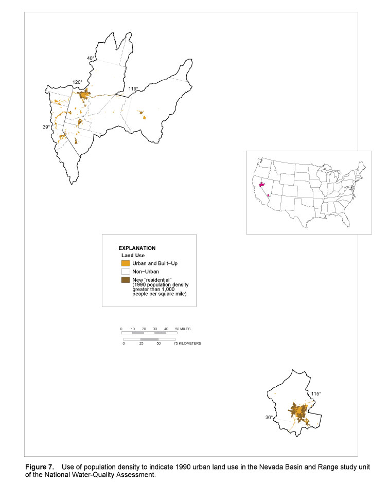
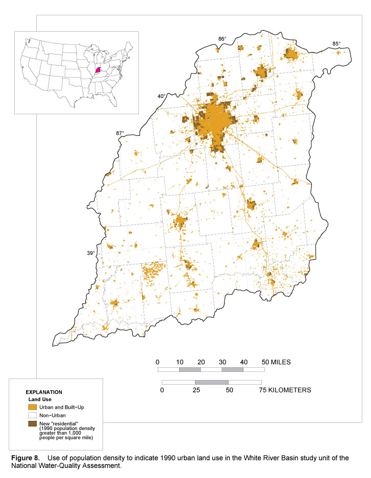
The technique for using population to define residential land use was applied to the first 20 NAWQA study units. The results for four of the study units are shown in figures 5-8. The maps of new "residential" land use show similar patterns of increased areas of "residential" land surrounding areas previously defined as "urban or built-up." This pattern is one that would be expected where suburban areas are expanding from a central urban core, which is illustrated by Atlanta, Georgia (Apalachicola-Chattahoochee-Flint study unit); Las Vegas, Nevada (Nevada Basin and Range study unit); and Indianapolis, Indiana (White River Basin study unit). The maps also show new "residential" land use where no urban or built-up land use existed previously. People in the NAWQA study units have verified that the results give reasonable indications of urbanization that has occurred in their study units since the 1970's land-use data were compiled.


The above classification system will enable NAWQA scientists to relate today's water quality information to recent georeferenced information on where people are living, rather than to data that are 20 years old. Water-quality information collected in NAWQA study units will be related to variables representing human and natural influences. Some of those will be population or housing densities, or information derived from those densities. For example, a study by Eckhardt and Stackelberg (1994) has shown that there are generally different concentrations of groundwater contaminants under low, medium, and high density residential areas of Long Island. As a second example, surface-water concentrations may be related to the percentage of the area upstream of the measuring site that is in each of the population classes. Long-term measurements of quality at one site may be directly related to the change in population density between the 1970's and 1990's, with concentrations of contaminants increasing as population has increased.
The use of population data to define residential land use has several limitations. First, it represents only one type of "urban" land use and does not account for the commercial, industrial, or transportation components of "urban" land use. However, refining these uses with other ancillary data besides population may be possible. Second, the density of population does not measure structures on the land; it measures only how many people are in a given area. Third, the assumptions about excluding urban and water categories of use when re-classifying polygons could introduce error. Although unlikely, urban areas possibly could have reverted to non-urban uses. Also, water areas possibly could have been converted to urban uses. Fourth, the procedure did not remove block groups coded as "water" in the TIGER/Line files. The procedure removed polygons coded as "water" in the land-use data. Last, assigning population density and the corresponding land use classification by entire block groups might over-represent the areal extent of new "residential" areas because the actual extent of the new "residential" area could be smaller than the whole block group.
Using this scheme based on population density, one can refine residential land use in any National Water-Quality Assessment study unit using the 1970's land use and 1990 population density. The technique gives a uniform definition of "residential" land use representative of the early 1990's timeframe that is useful in comparing and contrasting findings about water-quality in NAWQA study units.
Anderson, J.R., Hardy, E.E., Roach, J.T., and Witmer, R.E., 1976, A land use and land cover classification system for use with remote sensor data: U.S. Geological Survey Professional Paper 964, 28 p.
Bureau of the Census, 1990, TIGER: The coast-to-coast digital map data base: 18 p.
---------1991a, Census of population and housing, 1990: Public Law 94-171 data (United States) [machine-readable data files]: Washington, D.C., The Bureau [producer and distributor].
---------1991b, Census of population and housing, 1990: Public Law 94-171 data technical documentation: Washington, D.C., The Bureau.
---------1991c, TIGER/Line Census Files, 1990 [machine-readable data files]: Washington, D.C., The Bureau [producer and distributor].
---------1991d, TIGER/Line Census Files, 1990 technical documentation: Washington, D.C., The Bureau, 63 p.
Eckhardt, D.A.V., and Stackelberg, P.E., 1995, Relation of ground-water quality to land use on Long Island, New York: Ground Water Journal, v. 33, no. 6, p. 1019-1033.
Fairfax County, Virginia, 1990, Concept for future development and land classification system, 74 p.
Helsel, D.R., and Hirsch, R.M., 1992, Statistical methods in water resources: New York, Elsevier, p. 276.
Leahy, P.P., Rosenshein, J.S., and Knopman, D.S, 1990, Implementation plan for the National Water-Quality Assessment Program: U.S. Geological Survey Open-File Report 90-174, 10 p.
Leahy, P.P., and Thompson, T.H., 1994, National Water-Quality Assessment Program, U.S. Geological Survey Open-File Report 94-70, 4 p.
Long Island Regional Planning Board, 1992, Quantification and analysis of land use for Nassau and Suffolk Counties, 1981: Hauppauge, N.Y., 47 p.
Mynar, F., II, and Hewitt, M. J., III, 1989, Population estimation for risk assessment: A comparison of methods, in ESRI User Conference, 9th annual meeting, Palm Springs, California, May 22-26, 1989, Proceedings: Redlands, Calif., Environmental Systems Research Inc., 7 p. [Each article separately paged.]
Tasker, G.D., and Driver, N.E., 1988, Nationwide regression models for predicting urban runoff water quality at unmonitored sites: Water Resources Bulletin, vol. 24, no. 5, p. 1091-1101.
U.S. Geological Survey, 1990, Land use and land cover digital data from 1:250,000- and 1:100,000-scale maps, Data user guide 4: Reston, Va., U.S. Geological Survey, 25 p.
Vesterby, M., Heimlich, R.E., and Krupa, K.S., 1994, Urbanization of rural land in the United States, Agricultural Economic Report No. 673, 59 p.
| Multiply | by | To obtain |
| mile | 1.609 | kilometer |
| square mile | 2.590 | square kilometer |
| acre | 4,047 | square meter |
| people per square mile | 0.386 | people per square kilometer |