Sustainability of Ground-Water Resources--Circular 1186
The markedly different response of confined and unconfined aquifers to pumping (before the ground-water system returns to a new equilibrium) is demonstrated by calculations of drawdown resulting from a single pumping well in an idealized example of each type of aquifer (Figures A-1 and A-2). The numerical values used in the calculations are listed in Table A-1. Inspection of these values indicates that they are the same except for the storage coefficient S. Herein lies the key, which we discuss further in this section. To a hydrogeologist, the values in Table A-1 indicate a moderately permeable (K) and transmissive (T) aquifer, typical values of the storage coefficient S for confined and unconfined aquifers, and a high rate of continuous pumping (Q) for one year (t).
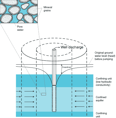
Figure A-1. Pumping a single well in an idealized confined aquifer. Confined aquifers remain completely saturated during pumping by wells (saturated thickness of aquifer remains unchanged)
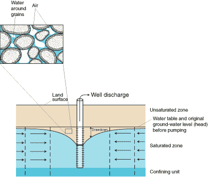
Figure A-2. Pumping a single well in an idealized unconfined aquifer. Dewatering occurs in cone of depression of unconfined aquifers during pumping by wells (saturated thickness of aquifer decreases).
A mathematical solution was developed by Theis (1940) to calculate drawdowns caused by a single well in an aquifer of infinite extent where the only source of water is from storage. This solution was used to calculate drawdowns at the end of one year of pumping for the confined and unconfined aquifers defined by the values in Table A-1. These drawdowns are plotted on Figure A-3. Inspection of Figure A-3 shows that drawdowns in the confined aquifer are always larger than drawdowns in the unconfined aquifer, and that significant, or at least measurable, drawdowns occur at much larger distances from the pumping well in the confined aquifer. For example, at a distance of 10,000 feet (about 2 miles) from the pumping well, the drawdown in the unconfined aquifer is too small to plot in Figure A-3, and the draw-down in the confined aquifer is about 10 feet. Furthermore, a measurable drawdown still occurs in the confined aquifer at a distance of 500,000 feet (about 95 miles) from the pumping well. Considering this information in a spatial sense, the cone of depression (Figure A-4) associated with the pumping well in the confined aquifer is deeper and much more areally extensive compared to the cone of depression in the unconfined aquifer. In fact, the total volume of the cone of depression in the confined aquifer is about 2,000 times larger than the total volume of the cone of depression in the unconfined aquifer for this example of a hypothetical infinite aquifer.
| Table A-1. Numerical values of parameters used to calculate drawdowns in ground-water levels in response to pumping in two idealized aquifers, one confined and one unconfined | ||
| Parameter | Confined aquifer | Unconfined aquifer |
| Hydraulic conductivity, K |
100 feet per day
|
100 feet per day |
| Aquifer thickness, b | 100 feet | 100 feet |
| Transmissivity, T | 10,000 feet squared per day | 10,000 feet squared per day |
| Storage coefficient, S | 0.0001 | 0.2 |
| Duration of pumping, t | 365 days | 365 days |
| Rate of pumping, Q |
192,500 cubic feet per day (1,000 gallons per minute) |
192,500 cubic feet per day (1,000 gallons per minute) |
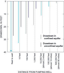
Figure A-3. Comparison of drawdowns after 1 year at selected distances from single wells that are pumped at the same rate in an idealized confined aquifer and an idealized unconfined aquifer. Note that the distances on the x-axis are not constant or to scale.
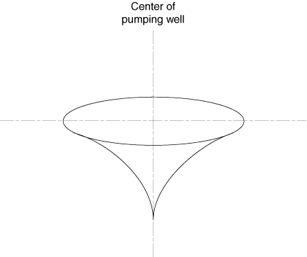
Figure A-4. The cone of depression associated with a pumping well in a homogeneous aquifer.
The large differences in drawdowns and related volumes of the cone of depression in the two types of aquifers relate directly to how the two types of aquifers respond to pumping. In unconfined aquifers (Figure A-2) dewatering of the formerly saturated space between grains or in cracks or solution holes takes place. This dewatering results in significant volumes of water being released from storage per unit volume of earth material in the cone of depression. On the other hand, in confined aquifers (Figure A-1) the entire thickness of the aquifer remains saturated during pumping. However, pumping causes a decrease in head and an accompanying decrease in water pressure in the aquifer within the cone of depression. This decrease in water pressure allows the water to expand slightly and causes a slight compression of the solid skeleton of earth material in the aquifer. The volume of water released from storage per unit volume of earth material in the cone of depression in a confined aquifer is small compared to the volume of water released by dewatering of the earth materials in an unconfined aquifer. The difference in how the two types of aquifers respond to pumping is reflected in the large numerical difference for values of the storage coefficient S in Table A-1.
The idealized aquifers and associated calculations of aquifer response to pumping discussed here represent ideal end members of a continuum; that is, the response of many real aquifers lies somewhere between the responses in these idealized examples.