U.S. DEPARTMENT OF THE INTERIOR
U.S. GEOLOGICAL SURVEY
CRUISE REPORT
RV INLAND SURVEYER CRUISE IS-98
THE BATHYMETRY OF LAKE TAHOE, CALIFORNIA-NEVADA
August 2 through August 17, 1998
Lake Tahoe, California and Nevada
James V. Gardner 1, Larry A. Mayer 2 , and John Hughes-Clarke 2
Open-File Report 98-509
Conducted under a Cooperative Agreement between the US Geological Survey and the Ocean Mapping Group, University of New Brunswick
This report is preliminary and has not been reviewed for conformity with U.S. Geological Survey editorial standards or with the North American Stratigraphic Code. Use of trade, product, or firm names in this report is for descriptive purposes only and does not imply endorsement by the U.S. Government.
1 U.S. Geological Survey, MS 999 345 Middlefield Road, Menlo Park, CA
94025
2 Ocean Mapping Group, University of New Brunswick, Fredericton, NB E3B
5B3
![]()
THE BATHYMETRY OF LAKE TAHOE, CALIFORNIA-NEVADA
The major objective of cruise IS-98 was to map the bathymetry of Lake Tahoe, California-Nevada (Fig. 1) to fulfill a commitment made during the Lake Tahoe Presidential Forum in 1997. The only existing bathymetry of Lake Tahoe, collected in 1923, was recently compiled by Rowe and Stone (1997), but the data density is inadequate for the level of scientific studies ongoing and anticipated in the near future for Lake Tahoe. Recent advances in marine multibeam-sonar capabilities now permit a cost-effective way, to precisely map the bathymetry of large areas of the ocean floor with 100% coverage. Cruise IS-98 applied this state-of-the-art ocean technology to Lake Tahoe. The newest of these high-resolution multibeam mapping systems also simultaneously collects backscatter (similar to sidescan sonar) imagery that results in a complimentary and co-registered data set that is related to the distribution of lake-floor materials and textures. The two types of maps that resulted from this cruise provide the multidisiplinary Lake Tahoe research community an unprecedented set of base maps upon which to build their studies. This report describes the high-resolution multibeam mapping system used at Lake Tahoe, outlines the data-processing steps used to produce the maps, and includes the daily log of the cruise.
The Kongsberg Simrad EM1000 High-Resolution Multibeam Mapping System
There are several different brands of high-resolution multibeam mapping systems that are appropriate for shallow-water surveys. After a review of the currently available systems, we chose to use the Kongsberg Simrad EM1000 system because of its proven track record, its demonstrated portability, its ability to map large areas at high speed without compromising data quality and, most importantly, its ability to simultaneously produce high-resolution side-scan sonar imagery. For the Lake Tahoe survey, we used an EM1000 system owned and operated by C&C Technologies, Inc. (Lafayette, LA) installed aboard the 26-ft Inland Surveyor (Fig. 2).
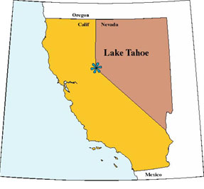 |
Figure 1. Location map of Lake Tahoe, California-Nevada |
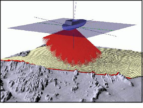
An overview of high-resolution multibeam mapping systems can be found in Hughes-Clarke, et al. (1996). The Simrad EM1000 system operates at a frequency of 95 kHz from a semi-circular transducer that is mounted on a rigidly attached ram on the bow of Inland Surveyor. The system was designed to operate in several modes through a range of depths from 5 to approximately 800-m water depth. The shallow (ultrawide) mode, used to maximum depths of about 200 m, forms 60 receive beams with a spacing of 2.5° distributed across track and 3° wide along track. This geometry generates a 150° swath that covers 7.4 times the water depth (Fig. 3). The wide mode, used to maximum depths of about 600 m, uses 48 formed beams with a spacing of 2.5 ° that results in a swath of 120° or 3.4 times the water depth. The deep mode, for water depths greater than 500 m, uses 48 formed beams with a spacing of 1.25° that generates a swath of 60° or 1.1 times the water depth. There are options within these modes for beam distribution (equiangular or equidistant) and pulse lengths. The specific options used for the Lake Tahoe survey are discussed in the data processing section below.
Most conventional vertical-incidence echo sounders determine the time of arrival of the returned pulse (and thus the depth) by detecting the position of the sharp leading edge of the returned echo, a technique called amplitude detection. In multibeam sonars, where the angle of incidence increases for each consecutive receive beam to either side of the vertical (nadir), a returned echo loses its sharp leading edge and the accurate determination of depth becomes inaccurate. To address this problem, the EM1000 multibeam system uses an interferometric principle in which each beam is split, through electronic beamforming, into two "halfbeams" and the phase difference between these "halfbeams" is calculated to provide a measure of the angle of arrival of the echo. The point at which the phase is zero (i.e., where the wavefront of the returned echo is normal to the receive-beam bore) is determined for each beam and provides an accurate measure of the range to the seafloor. Both amplitude and phase detection are recorded for each beam and then the system software picks the "best" detection method for each beam, based on a number of quality measurements, and uses this method to calculate depth.
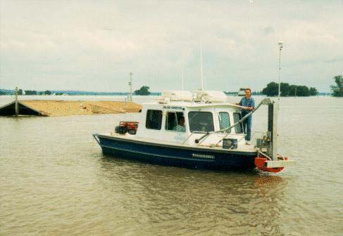 |
Figure 2. Inland Surveyor with Kongsberg Simrad EM1000 mounted on bow. |
|
| Figure 3. Cartoon of multibeam receive cycle showing 60 beams spread over 150° swath. |
The EM1000 also provides quantitative seafloor-backscatter data that can be displayed in a sidescan-sonar-like image. The backscatter images can be used to gain insight into the spatial distribution of seafloor properties. A time series of echo amplitudes from each beam is recorded at 0.2- to 2.0-ms sampling rate, depending on the water depth. The echo amplitudes are sampled a much faster rate than the beam spacing and can be processed from beam-to-beam to produce a backscatter image with the theoretical resolution of the sampling interval (15 cm at 0.2 ms). The amplitude information can be placed in its geometrically correct position relative to the across-track profile because the angular direction of each range sample is known. The EM1000 software corrects the amplitude time series for gain changes, propagation losses, predicted beam patterns and for the insonified area (with the simplifying assumptions of a flat seafloor and Lambertian scattering). Subsequent processing (see below) uses real seafloor slopes and applies empirically derived beam-pattern corrections to produce a quantitative estimate of seafloor backscatter across the swath.
In addition to the multibeam sonar array, a multibeam survey requires a careful integration of a number of ancillary systems. These include: (1) a differentially corrected Global Positioning System (DGPS); (2) an accurate measure the heave, pitch, roll, and heading of the vessel, all to better than 0.01° and the transformation these measurements to estimates of the motion of the transducer at the times of transmission and reception (motion sensor); (3) a method to precisely determine the sound-speed structure of the water column, using measurements of temperature, salinity and depth with a CTD and the calculation of sound velocity profiles [SVP].
The Lake Tahoe survey was navigated with inertial positioning provided by an Applied Analytic POS/MV motion sensor as well as a Trimble DGPS. The POS/MV records vehicle motion at 100 Hz with an accuracy of 0.01°. USGS benchmarks were located at two sites on the north end of Lake Tahoe and their positions were determined with a DGPS. These provided a local calibration for a position accuracy for the survey of ±1 m.
Sound-velocity profiles were calculated several times each day so that ray-tracing techniques could be used to determine the effect of acoustic refraction in the water, principally caused by variations in water temperature. A SeaBird CTD was deployed the first day of operations to get a good reference SVP. Sippican T-7 expendable bathythermographs (0 to 600-m water depth) were routinely collected anytime it was suspected that the water structure had changed during the course of the survey. An additional sound-velocity profiler is installed at the transducer array to determine the speed of sound in water directly at the transducer. All the SVP data are fed directly into the Simrad EM1000 processor for instantaneous beamforming and raytracing of the individual beams.
Raw EM1000 data telegrams were acquired over an ethernet on a shipboard workstation. The data stream include is shown in Table 1. A number of ancillary data sources were also acquired by C&C Technologies (Table 2).
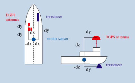 |
Figure 4. Measured offsets required for accurate pitch, roll, yaw, and position. |
Table 1. Kongsberg Simrad EM1000 data stream.
|
Table 2. Ancillary data sources
|
The accurate reduction of swath bathymetric data critically depends on a proper knowledge of the geometry and relative positions of the sonar transducer with respect to the motion sensor, the ship, and the positioning-system antennae (Fig. 4). C&C Technologies, using standard surveying techniques, measured these values before the survey began (Table 3). The transducer is at 1.3-m depth (vessel stationary). All values are relative to the transducer.
| Table 3. Offsets to sensor alignments on Inland Surveyor | |
| Sonar to IMU misalignment | |
| X mounting angle Y mounting angle Z mounting angle |
0.00° 0.30° 3.00° |
| Ship to IMU misalignment | |
| X mounting angle Y mounting angle Z mounting angle |
0.00° 0.30° 3.00° |
| IMU to sonar level arm | |
| X lever arm Y lever arm Z lever arm |
171 cm 0.00 cm 65 cm |
| IMU to GPS lever arm | |
| X lever arm Y lever arm Z lever arm |
-186 cm 0.00 cm -238 cm |
Three Vertical Reference Units were available onboard the Inland Surveyor to measure the pitch, roll, and yaw. The POS/MV, a full DGPS-aided inertial navigational system, was used as the primary attitude sensor and directly interfaced to the Simrad EM1000 and provided 100-Hz measurements of boat attitude to 0.01°. The POS/MV was chosen because it has high accuracy specifications, it is insensitive to long period horizontal accelerations, and it provides an inertial position solution that is reliable through DGPS outages of periods of less than about 1 or two minutes.
There are several operational modes available for the EM1000. The differences in the modes are a function of pulse length, beam spacing, and angular sector. The pulse length controls the amount of energy transmitted into the water column. The system can be operated in an "equiangular" (EA) mode in which the beams are spaced at equal angles apart, resulting in a non-linear (increasing spacing away from nadir) spacing of sonar footprints on the seafloor. The system can also be operated in an "equidistant" (EDBS) mode in which the beams are spaced such that the sonar footprints are equally spaced in the across-track profile. The EDBS geometry is achieved by generating variable beam-angular spacings. Although EDBS has advantages in data handling (i.e., provides even sounding density), there are two limitations. The beams in the 140° and 150° modes are spaced wider than their beam widths and results in incomplete coverage that produces a striping close to nadir. This problem disappears as the swath width closes to ~120°. However, the second limitation occurs because of attitude uncertainties and imperfect refraction models that can result in sounding errors that grow with angle from the vertical. Consequently, these limitations render the outermost beams less reliable than for the EA mode.
For the reasons stated above, the EA mode was used for the Lake Tahoe survey. In the EA mode, the EM1000 was operated with a 0.2 ms pulse length in waters less than 150 m deep, that provided a 150° swath. In waters deeper than 150 m, the EM1000 was operated with a 0.7 ms pulse length that generated a 120° swath.
Bathymetry
All bathymetric data were adjusted through Kongsberg Simrad software for (1) transducer draft, (2) static roll, pitch and gyro misalignments, (3) pitch on transmit, (4) heave at transmit and reception, (5) roll at reception, (6) refracted ray path, and (7) beam steering at transducer interface. Post-logging transformations included (1) transformation of navigation from antenna to transducer, (2) correction for positioning to sonar time shifts, (3) lake surface elevation, and (4) any unaccounted for static attitude misalignments.
Backscatter
The Kongsberg Simrad EM1000 provides a backscatter-intensity time series for the bottom insonification period for each of the 60 individual beams. The corrections applied by the shipboard recording system are listed in the table below in Table 4.
A set of required transformations are performed by specialized software written by the Ocean Mapping Group at the University of New Brunswick. These transformations include conversion of each beam time series to a horizontal range equivalent, splicing the 60 beam traces together to produce one full slant-range corrected trace, and removal of residual beam-pattern effects. Although the system software corrects for average beam pattern, there are ± 2 dB ripples in the average beam pattern that vary from transducer to transducer. The beam pattern of the C & C EM1000 may be slightly different each time the stave connectors are reconnected in the transceiver.
Table 4. Corrections applied to each beam for backscatter.
|
Our processing approach to backscatter was to stack several thousand pings to view the angular variation of received backscatter intensity as a function of beam angle. Inherent in this function is both the transmit and receive sensitivities, as well as the mean angular response of the seafloor. We then invert this function to minimize the beam pattern and angular variations.
Kongsberg Simrad uses a variable gain within 15° of vertical to reduce logged dynamic range. The sidescan data at this stage have had a Lambertian response backed out and the beam pattern has been corrected with respect to the vertical and all receive beams have been roll stabilized. Consequently, corrections have been made for variations in the beam-forming amplifiers but not variations in the stave sensitivities of the physical array.
Additional transformations were required to produce calibrated backscatter measurements. These include (1) removal of Lambertian model, (2) true lake-floor slope correction, (3) refracted ray path correction, (4) residual beam pattern correction, and (5) aspherical-spreading corrections.
Despite the careful measurements of transducer alignments and offsets, the true geometry of the installed system can only be determined through the determination of the self-consistency of seafloor measurements. To facilitate such a determination, we conducted a series of "patch tests" in Lake Tahoe whereby the system was run back and forth across various features on the lake floor to determine if there were residual roll, pitch, heading, or timing offsets that required corection factors.
A full patch test procedure was started prior to data collection on August 2 to calibrate any time delay, and gyro misalignment. The static adjustments were estimated from the patch test are listed in Table 5.
Table 5. Adjustments to shipboard alignments used for Lake Tahoe survey
|
The 1-Hz DGPS data were logged with the Kongsberg Simrad EM1000 software. The Simrad Bottom Detection Unit (BDU time stamps the depth and sidescan telegrams and was slaved to a shipboard SUN Sparc 20 that itself was synched to the GPS 1 PPS. The navigation telegrams were externally stamped by the Trimble 4000 GPS receiver. The receiver antenna positions were shifted to the transducer according to the X and Y offsets using the POS/MV output.
Every 1-Hz navigation fix was checked for gross time and/or distance jumps by graphical examination during data processing. Outliers were interactively interrogated for time, flagged and rejected (or re-accepted). All navigation jumps greater than 20 s were automatically flagged as uninterpolatable.
Land-based data processing (Fig. 5) consisted of (1) the editing the 1-Hz navigation fixes to flag bad fixes; (2) examining each ping of each beam to flagg outliers, bad data, etc.; (3) merging the depth and backscatter data with the cleaned navigation; (4) reducing all depth values to mean lake level (1899 m); (5) performing additional refraction corrections, if necessary, for correct beam raytracing; (6) separating out the amplitude measurements for conversion to backscatter; (7) gridding depth and backscatter into a geographic projection at the highest resolution possible with water depth; (8) regridding individual subareas of bathymetry and backscatter into final georeferenced map sheets; (9) gridding and contouring the bathymetry; and (10) generation of the final maps. Nearly finalized maps were completed in the field one day after the completion of the cruise and the final maps that accompany this report were completed one week after the end of the cruise.
All swath bathymetric data were passed through a number of simple filters that flagged all beams that form a spike when compared to their neighbors for which the across-track slope anomalies exceed 25° and flagged all beams that form a spike when compared to their neighbors for which the along-track slope anomalies exceed 55°. These two criteria removed the worst of the spikes. All beams without immediate neighbors fore and aft were rejected and all beams without immediate neighbors port and starboard were rejected. The two criteria removed isolated beams but the remaining outliers had to be examined and subjectively examined using the UNB/OMG SwathEditor tool in a line by line mode.
|
Figure 5. Data processing flow chart. |
The single biggest limitation on the quality of sounding data is water-column refraction. Refraction-related anomalies grow non-linearly with beam angle and the resulting artifacts can create short-wavelength topographic features that may be misinterpreted as seabed geology. There was some fear voiced that the suspected strong lake stratification would present a problem for the beam steering and ray tracing of individual beams. This did not prove to be the case and the thermocline and density structure, as repeatedly measured by CTD and XBT, remaimed remarkable constant over the 16 days of the survey. A representative plot of a water-velocity profile is shown in Figure 6. In fact, no additional emperical refraction corrections were necessary during processing. If all of the alignments were correctly determined, Kongsberg Simrad states that depth "...accuracies better than 0.5% of water depth are achieved across the entire swath."
A lake-elevation station, located on the Coast Guard pier in Tahoe City, is maintained by the USGS. Readings are taken every four hours so that a detailed time series was available for the elevation of the lake surface relative to mean sea level. The lake elevation on August 2nd was 1899.08 m and on August 17th it was 1899.02 m. A lake elevation of 1899 m was used as the reference datum for all depth determinations. However, it appears that there may be a 0.43-m offset between the datum used for the elevation and the NGVD datum (Gerald Rockwell, personal commun., 1998). The lake level dropped only 6 cm over the duration of the mapping survey, but because the drop and the potential datum offset are smaller than the resolution of the system, so we did not adjust the depth determinations for these offsets. Once each lake depth determination was calculated, the value was converted to meters above mean sea level. This allows the entire Tahoe bathymetry to be merged with the regional DEM and to be viewed as a topographic feature.
 |
| Figure 6. Sound-velocity profiles collected throughout the Lake Tahoe survey. |
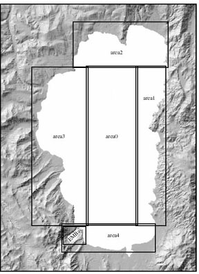
The large overview maps of backscatter and shaded relief that accompany this report were generated from larger-scale subarea maps (Fig. 7 and Table 6). The higher-resolution subarea maps were regridded at 10 m to produce the maps of the entire lake (Figs. 7 and 8). This regridding loses resolution in the shallower areas but allows the entire area to be mapped. The detailed subarea maps were produced at the maximum resolution allowable for the data.
Table 6. Mapsheet sizes in columns (cols), rows, in pixels and resolution (resol) in meters
BATHYMETRY |
BACKSCATTER | ||||||
| Mapsheets | columns |
rows |
resolution |
columns |
rows |
resolution | |
| Area0 Area1 Area2 Area3 Area4 EMBay |
661 |
2044 |
12 |
1322 |
4088 |
6 | |
Contour maps represent the more traditional method of displaying bathymetry. The contours were derived from the gridded elevations. The resultant contours were smoothed by a 3-point running average in the overview maps. Even at the original contour grid, more than 90% of the data have to be discarded so as to only show some chosen contour interval. A much better representation of bathymetry, using 100% of the data is a shaded-relief map.
|
| Figure 7. Map sheets used to process at highest resolution. See Table 6 for details. |
 |
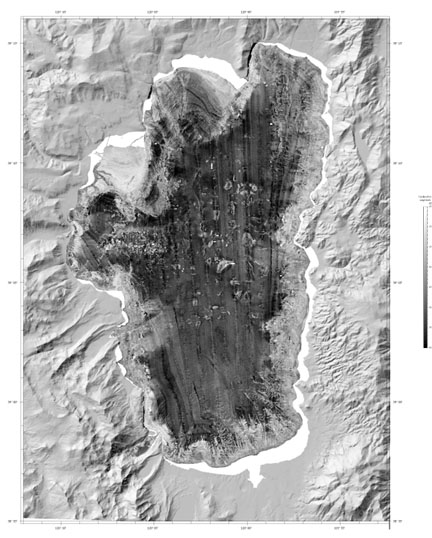
Figure 8. Shaded-relief bathymetry of Lake Tahoe. |
 |
| Figure 9. Backscatter (at 95kHz) of Lake Tahoe |
A shaded-relief map (Fig. 8) is a pseudo-sun-illumination of a topographic surface using the Lambertian scattering law (equation 1), where SI is the pseudo-sun intensity, K is a constant that allows for even background, and phi is the angle between the pseudo sun and
SI = K * cos phi (Eq. 1)
the bathymetric surface.
The backscatter map (Fig. 9) is a representation of the amount of acoustic energy, at 95 kHz, that is scattered back to the receiver from the lake floor. The Kongsberg Simrad EM1000 system has been calibrated at the factory and all gains, power levels, etc. that are applied during signal generation and detection are recorded for each beam and are used to adjust the amplitude value prior to recording. Consequently, the backscatter is calibrated to an absolute reflectance of the seabed. However, the amount of energy, measured in decibels (dB), is some complex function of constructional and destructional interference caused by the interaction of an acoustic wave with a volume of sediment or, in the case of hard rock, the rock material. The backscatter from sediment is volume reverberation to at least 10 cm caused by seabed and subsurface interface roughnesses above the Rayleigh criteria (a function of acoustic wave length), the composition of the sediment, and its bulk properties (water content, bulk density, etc.). Although, it is not possible to determine a unique geological facies from the backscatter value, reasonable predictions can be made from the backscatter based on the local geology.
It can not be stressed too strongly that one of the great advantages of this survey is that the bathymetry is completely georeferenced with the backscatter. Consequently, each pixel on the map has a latitude, longitude, depth, and backscatter value assigned to it.
August 3, 1998 (980803)
The C&C Technology team arrived in Tahoe City and the RV Inland Surveyor
was launched at the boat ramp adjacent to the Coast Guard station. The rest
of the day was spent on the water performing patch tests to ensure all the
system alignments were correct. A 3° yaw offset was noticed, but the
other systems appeared aligned. It was determined that the EM1000 could
be run in the shallow and medium modes for optimum resolution and the deep
mode is not required. Weather and lake-state conditions were ideal for the
survey. One surprise was that the measured sound speed at the transducer
(~1-m deep) was 1484 m/s, as measured by both velocity sensors at the transducer.
A Seabird CTD was run to ~200 m depth and the sound speed decreased to a
minimum at 50 m of ~1428 m/s.
A second surprise was that the 1900-m elevation of Lake Tahoe rendered the engines of Inland Surveyor less efficient than was predicted. The result of this inefficiency was that a maximum speed of only ~8 kts could be maintained. A new set of propellers was ordered to increase speed.
C&C located two USGS benchmarks around the lake and calibrated their navigation systems with ease. The Coast Guard measures the lake elevation (to the nearest millimeter) once a day and agreed to provide me with those measurements. These data provided our "tides" for producing corrected elevations for the lake floor.
August 4, 1998 (980804)
John Hughes-Clarke spent the day on the boat conducting additional patch
tests. A USGS benchmark (Tavern Hole) was located on the west side of the
lake for an additional navigation reference. By noon the systems were operating
at normal levels so the survey began with a complete circumnavigation of
the lake following the 100-m isobath. This survey provided the necessary
baseline for separating the medium from shallow modes. No problems were
encountered and the afternoon winds did not materialize.
August 5, 1998 (980805)
Routine day of data collection and processing. It was discovered on the
last line of day 980804 that the POS/MV offsets were not properly set in
the software. Consequently, we built a new script (unravel.special) only
for day 980804 and reprocessed the entire days data. An additional line
was inserted in mergeNav (-declin -3.0) and a new line was added to the
script (unrollOMG roll_offset -0.3 *.merged) for day 980804. The survey
circumnavigated the lake once again and returned back up the west side to
complete the day.
The sediments in the chutes between headlands and in small channels have such low backscatter (~-55 dB) that the EM1000 could not acquire bottom detect in the areas where the wall of the channel/chute meets the floor. The result was data dropouts and we could find no solution to this problem. It is a minor problem, but an interesting one. The new propellers arrrived and were installed at the end of the day.
August 6, 1998 (980806)
Routine day of data collection and processing. The correction for the POS
offset had to be adjusted again by the script unrollOMG roll_offset 0.3
*.merged for day 980805. All data for day 980805 were reprocessed. The survey
continued to fill in the deep areas of the lake. The new propellers did
not improve survey speed.
August 7, 1998 (980807)
Routine day of data collection and processing. Fresh breezes began blowing
at about 11:00 am and picked up to ~25 kts throughout the afternoon. This
caused a considerable amount of rolling and pitching on the boat, but the
data did not suffer at all.
August 8, 1998 (980808)
Routine day of data collection and processing. The boat crew discovered
that two offsets in the Simrad software were not properly set. The offset
between the POS/MV and the transducer should be +1.71 m but was set at +0.41
m. The timing offset should be +1.0 s but was set at +1.25 s. A quick calculation
shows that these two errors effectively cancel one another so we decided
not to change the settings, but instead will complete the survey with one
set of offset constants.
August 9, 1998 (980809)
Routine day of data collection and processing.
August 10, 1998 (980810)
Routine day of data collection and processing.
August 11, 1998 (980811)
Routine day of data collection and processing.
August 12, 1998 (980812)
The entire day was devoted to the news media and a visit by Secretary of
Interior, Mr. Bruce Babbitt. The day began at 7:00 am with an open house
for the press aboard the Inland Surveyor tied up at the Tahoe City
Marina. News media from San Francisco, San Jose, Sacramento, Reno, as well
as the local Lake Tahoe area, turned out. Promptly at 9:00 the Inland
Surveyer left the dock with Secretary Babbitt aboard and we surveyed
an area locally known as the tavern hole. At 10:00 Secretary Babbitt and
a host of news media visited the data processing center (Mission Control)
set up in a living room at the Tahoe Marina Lodge.
The afternoon was spent at a "stake-holders conference" where we presented the images on a large-screen TV connected to the Silicon Graphics workstation and answered questions. Toward the conclusion of this conference, we asked the stake holders what they wanted us to do with our remaining survey time. A consensus was reached that they wanted us to complete the mapping to the 20-m isobath.
While the conference was in session the Inland Surveyor returned to the lake and spent the afternoon continuing the survey.
August 13, 1998 (980813)
Routine day of data collection and processing until toward the end of the
day the computer aboard Inland Surveyor locked up and we lost all
of the days data before they weree backed up. The day's survey was repeated
the next day.
August 14, 1998 (980814)
Routine day of data collection and processing until the mid afternon. Violent
thunderstorms with lightning and hail pelted Lake Tahoe all afternoon. Torrential
rain occurred for 30 minutes but the lightning continued for two hours.
All processing computers in Mission Control were shut down for fear of a
power surge; consequently, very little could be accomplished during the
storm. The surveying continued during the storm until aboat 4:00 pm when
the storm's intensity dictated terminating the survey and a return to shore
for safety reasons.
August 15, 1998 (980815)
Routine day of data collection and processing. The basin of Lake Tahoe deeper
than about 50 m was completed. The shallow areas along the east and north
sides were mapped to at least the 20-m contour.
August 16, 1998 (980816)
Routine day of data collection and processing. The shallow areas along the
west side of the lake were mapped to at least the 20-m contour. The remaining
areas shoaler than 20 m along the western side of the lake is very difficult
to map because of the density of piers and moored boats.
August 17, 1998 (980814)
Routine day of data collection and processing. Around noon one of the outboard
motors of Inland Surveyor quit and it was determined that bad gas caused
the problem. New plugs and an additional fuel filter were added and the
survey continued with only an hour lost. The survey ended at 6:00 pm PDST.
All of the lake deeper than ~10 m was surveyed except for those areas with
piers or moored boats.
August 18, 1998 (980818)
The data from August 17th were processed and the final field maps were completed. The computers were packed and the field program ended.
Hughes Clarke, J.E., Mayer, L.A., and Wells, D.E., 1996, Shallow-water imaging multibeam somars: A new tool for investigating seafloor processes in the coastal zone and on the continental shelf. Marine Geophysical Researches, 18: 607-629.
Rowe, T.G. and Stone, J.C., 1997, Selected hydrographic features of the Lake Tahoe Basin, California and Nevada. U.S. Geol. Survey Open-File Rept. 97-384.
![]()