Data Series 892
Notice: This USGS Publication Supersedes Data Series 812
|
|||||||||||||||||||||||||||||||||||||||||||||||||||||||||||||||||||||||||||||||||||||||||||||||||||||||||||||||||||
| Station name | GTN-P code | Station installation | Latitude | Longitude | Elevation (m) |
|---|---|---|---|---|---|
|
1 Awuna1 was decommissioned on 22 May 2004. It was replaced by Awuna2, located 1.91 kilometers to the southwest. The two stations ran concurrently for several months. 2 Lake 145 has not yet been assigned a GTN-P code. |
|||||
| Drew Point | U20 | 18 AUG 1998 | 70°51.872′N. | 153°54.405′W. | 5 |
| Inigok | U21 | 17 AUG 1998 | 69°59.377′N. | 153°05.630′W. | 53 |
| Fish Creek | U22 | 18 AUG 1998 | 70°20.114′N. | 152°03.120′W. | 31 |
| Awuna11 | U23 | 19 AUG 1998 | 69°10.226′N. | 158°00.402′W. | 362 |
| Umiat | U24 | 20 AUG 1998 | 69°23.741′N. | 152°08.568′W. | 201 |
| Tunalik | U25 | 20 AUG 1998 | 70°11.756′N. | 161°04.687′W. | 26 |
| Koluktak | U30 | 27 AUG 1999 | 69°45.096′N. | 154°37.054′W. | 60 |
| South Meade | U33 | 08 AUG 2003 | 70°37.708′N. | 156°50.119′W. | 15 |
| Awuna2 | U35 | 22 AUG 2003 | 69°09.331′N. | 158°01.827′W. | 343 |
| Piksiksak | U37 | 08 AUG 2004 | 70°02.197′N. | 157°04.882′W. | 33 |
| East Teshekpuk | U38 | 10 AUG 2004 | 70°34.111′N. | 152°57.899′W. | 7 |
| Ikpikpuk | U39 | 21 AUG 2005 | 70°26.499′N. | 154°21.938′W. | 5 |
| Lake 1452 | — | 13 AUG 2007 | 70°41.388′N. | 152°37.995′W. | 6 |
| Niguanak | U29 | 18 AUG 2000 | 69°53.363′N. | 142°59.037′W. | 84 |
| Marsh Creek | U31 | 03 AUG 2001 | 69°46.657′N. | 144°47.595′W. | 260 |
| Camden Bay | U34 | 14 AUG 2003 | 69°58.317′N. | 144°46.234′W. | 4 |
| Red Sheep Creek | U36 | 03 AUG 2004 | 68°40.898′N. | 144°50.524′W. | 785 |

Historically, very little climate information has been collected on Federal lands in Arctic Alaska. The information that has been collected generally resulted from short-term campaigns designed to support oil development and other activities. This report provides data collected by the DOI/GTN-P climate monitoring array over the period August 1998 through July 2013 that greatly augment the existing record for this region. Variables presented in this report include ground temperature at 10 depths (5–120 cm), soil moisture, air temperature and pressure, wind speed and direction, incident and reflected solar flux, snow depth, and rainfall. Because the network took nearly a decade to develop (table 1), the records are of varying lengths. For example, the longest air and ground temperature and snow depth records cover nearly 15 years (as of July 2013), whereas the longest wind and soil moisture records cover about 10 years (table 2). Although short, the records are long enough to establish climate gradients and patterns across the region, quantify the magnitude of variability on daily through annual timescales, and provide the context for future climate change. Data collection is ongoing. Subsequent reports will provide annual updates and information on the full suite of climate variables monitored by the network.
Each station consists of a solar- and battery-powered datalogger (Campbell Scientific [CSI] model CR10X or CR1000, depending on the station), a sensor mast, and the sensors (fig. 2). Air temperature, wind, radiation and rainfall values are sampled every 30 seconds and then averaged once per hour (rainfall is totaled). Ground temperatures, soil moisture, snow depth, and surface pressure values are sampled once per hour. The resultant data stream from this sampling protocol is of hourly resolution. Because of limited power and data storage capacity, measurements taken before August 2003 were stored once every 2 hours rather than hourly. Physical site visits are made 1–2 times per year to collect the stored measurements and to perform station maintenance. For the stations with telemetry (table 1), data are occasionally downloaded between site visits.
The air temperature measurements are made using a Campbell Scientific CSI model 107 thermistor probe mounted in a naturally aspirated six-gill radiation shield located 3 meters (m) above the surface as measured during the snow-free period. The CSI model 107 probe is sampled using a half-bridge voltage measurement. To reduce measurement uncertainties, voltages are converted to temperature during the data processing step using a four-term calibration function appropriate for the full temperature range experienced at these sites (–50 °C to +30 °C).
Wind speed and direction are measured using a R.M. Young 05103 wind monitor, located 3 m above the surface. For wind direction, the hourly vector mean is stored, although prior to April 2008, the arithmetic mean was stored rather than the vector mean.
Ground temperature is measured once per hour at ten depths using a Measurement Research Corporation (MRC) TP101 model temperature probe. The probe is 125 cm long and contains 10 thermistors at depths of 5, 10, 15, 20, 25, 30, 45, 70, 95, 120 cm. The MRC thermistors are read on a single-ended channel through an interface circuit containing a half-bridge network and a means to switch the excitation voltage to each thermistor. A fixed precision resistor within the MRC is sampled at each time-step for comparison and to improve the estimate of the measurement voltages. Resistance is calculated from the voltage measurements and then converted to temperature using a four-term calibration function similar to the Steinhart-Hart equation (Steinhart and Hart, 1968) but with an additional term that improves the calibration fit below 0 °C.
Incident and reflected solar-flux measurements are made with CSI model LI200X silicon pyranometers located 3 m above the surface. The pyranometers are measured using a differential voltage measurement. A factory standard-calibration factor is applied to the resultant voltages to produce energy-flux values.
Rainfall is measured with a Texas Electronics TE 525 rain gage mounted approximately 60 cm above the ground in the middle of an ETI Instrument Systems Lexan altershield. The sensor is sampled every 30 seconds and millimeter totals are stored once per hour.
Snow depth is measured once per hour with a CSI model SR50 ultrasonic distance sensor mounted approximately 2.5 m above the ground surface. The sensor sends out an ultrasonic pulse and measures the time it takes for the signal to bounce off the ground or snow surface and return to the sensor. The travel time of the ultrasonic pulse varies with temperature; this effect is taken into account using data from the CSI model 107 air temperature sensor. The distance to the ground calculated from the ultrasonic travel time is subtracted from the known distance, as measured during physical site visits and distance-data analysis, to calculate snow depth.
Soil moisture is measured once per hour at approximately 15-cm depth using a Stevens Hydra Probe Soil Moisture sensor. Four single-ended voltage measurements are stored by the datalogger and then converted to soil moisture and salinity using algorithms supplied by the manufacturer.
Atmospheric pressure is measured once per hour through a vented port in the datalogger enclosure using a Vaisala PTB101B barometer.Because of the harsh operating environment, a variety of problems can affect the sensors and resulting data streams. These include loss of system power, total or partial failure of the sensor-support mast due to bear activity, damage or destruction of sensor cables or the sensors themselves by wildlife, obstruction of air temperature radiation shields by snow or rime ice, complete freeze-up of wind sensors by rime ice, obstruction of incident solar-flux detectors by snow, corrosion of snow depth transducers by high humidity, false snow depth signals caused by blowing snow, intermittent electrical noise associated with electric bear fences, vertical movement ("jacking") of ground temperature sensors by freeze-thaw forces, and others.
A multi-component data-processing system has been developed to automatically and consistently handle a number of the data processing tasks, including application of sensor calibration factors, masking data during periods that are known to be problematic, masking data that are outside reasonable predefined limits, calculation of derived climate variables (for example, thawing-degree days, maximum active-layer depth, and total precipitation), calculation of climate statistics on a variety of timescales (hourly to decadal), and calculation of climate trends and anomalies. Predefined faulty data limits are unique to each sensor and are based on known environmental extremes and sensor specific performance. For example, hourly average wind speed values are flagged for masking if they are less than zero (physically impossible) or if they exceed 40 m s-1 (meter per second), a condition that is highly unlikely. The system also includes a number of tools to assist the data technician in identifying spurious data that are missed by the automated routines and require a higher level of analysis. For example, wind speed values are automatically flagged if they do not change for 6 consecutive hours, likely indicating a condition of sensor freeze-up during icing. The technician is notified of these periods and directed to investigate each freeze-up period individually for any additional masking that may be necessary. First, the processing system is applied on a station and sensor-specific basis. Second, the system is used in interstation mode, whereby statistics are calculated for data from the one or two most spatially proximate stations, depending on data availability and environmental homogeneity. Time periods that contain data that exceed statistical limits are further scrutinized and masked where appropriate. Details of the data processing system are described in "DOI/GTN-P Climate-Station Data, Quality Assurance and Control Procedures" (G.D. Clow and F.E. Urban, unpub. data, 2012).
The resistance Rs of a CSI model 107 air temperature sensor is determined from the stored half-bridge voltage V using the equation
![]() where Rf and Rb are the resistances of the field and bridge resistors in the half-bridge, respectively, and Vx is the excitation voltage. The excitation voltage can vary slightly, so it is collected each time a measurement is made. Temperature is then calculated from the measured resistance using the four-term calibration function
where Rf and Rb are the resistances of the field and bridge resistors in the half-bridge, respectively, and Vx is the excitation voltage. The excitation voltage can vary slightly, so it is collected each time a measurement is made. Temperature is then calculated from the measured resistance using the four-term calibration function
![]() where T is temperature expressed in Kelvin. This is an extension of the often used Steinhart-Hart equation (Steinhart and Hart, 1968), which proved inadequate for our purposes below 0 °C. The four calibration coefficients (a0, a1, a2, a3) are determined for each CSI model 107 probe by monitoring its resistance while the temperature is varied from –50 °C to +30 °C in a Hart Scientific temperature calibration bath at the USGS temperature calibration facility in Lakewood, Colorado. For those rare instances where a0, a1, a2, a3 are unavailable for a particular CSI model 107 sensor, we use values that have been determined for a "factory standard" probe.
where T is temperature expressed in Kelvin. This is an extension of the often used Steinhart-Hart equation (Steinhart and Hart, 1968), which proved inadequate for our purposes below 0 °C. The four calibration coefficients (a0, a1, a2, a3) are determined for each CSI model 107 probe by monitoring its resistance while the temperature is varied from –50 °C to +30 °C in a Hart Scientific temperature calibration bath at the USGS temperature calibration facility in Lakewood, Colorado. For those rare instances where a0, a1, a2, a3 are unavailable for a particular CSI model 107 sensor, we use values that have been determined for a "factory standard" probe.
Temperature measurements are assigned a bad data code when it is determined they do not represent the air temperature field 3 m above the ground. Data that have been assigned such a code are effectively masked and are not used in any further calculations (for example, climate statistics, climate trends, or climate anomalies). Beyond the general problems described above (for example, insufficient system power and change in sensor height due to sensor mast damage), specific problems that can lead to air temperature masking include (a) reduction of the necessary ventilation through the radiation shield by snow, rime ice, or low wind speeds (<1 m s-1 [meter per second]), and (b) the sensor falling out of the radiation shield, exposing it to solar radiational heating. Air temperature climate statistics are calculated when the data are available at least 95 percent of the time.
No calibration factors or corrections are currently applied to the wind speed or wind direction measurements. Specific problems that can lead to masking of either the wind speed or wind direction include significant ice buildup that prevents the wind monitor from functioning properly. In some cases, icing will affect the wind speed measurements but not the wind direction, and vice versa. The threshold for calculating climate statistics for the wind variables is the same as for air temperature, that is, 95 percent data availability.
The resistances of the MRC TP101 thermistors are determined from the stored half-bridge voltages using known values for the excitation voltage and the circuit's fixed resistors. The thermistor resistances are then converted to temperature using the same four-term calibration function (eq. 2) as for the air temperature sensor. In this case, the four calibration coefficients (a0, a1, a2, a3) were determined from data for a "factory standard" MRC probe over the temperature range –40 to +10 °C. The stated uncertainty of the MRC measurements is 0.1 °C. To further reduce the uncertainty of the ground temperature measurements, a special set of orthonormal basis functions were fit to the mean-annual ground temperature profiles in a least-squares sense where the number of basis functions retained was determined by the reduced chi-squared values. The difference between the mean-annual temperature profiles (based on the factory standard calibration) and the resulting least-squares fit provided an estimate of the unique calibration offset for each thermistor relative to the factory standard. These calibration offsets were then applied as corrections to the data. With these corrections, the standard uncertainty of the ground temperature measurements is believed be in the range 0.02–0.05 °C. Beyond the general system problems (power loss, sensor or sensor cable damage, and so forth) that can lead to masking, the ground temperature instrument is subject to freeze-thaw processes inherent to its placement in permafrost. The MRC is a rigid instrument (the thermistors are encased in a hard epoxy potting in a long cylindrical shape), and permafrost and freeze-thaw processes periodically act to "jack" the instrument vertically out of its original position. The amount of "jacking" varies widely year to year and among stations. Many sites experienced no jacking, some experienced small (1–3 cm) documented amounts, and several experienced extreme (5–10 cm) amounts. The data processing system is used to mask data from the topmost thermistors at the 5- and sometimes 10-cm depths when their values during unfrozen time periods exceed local air temperatures. These criteria indicate that portions of the instrument are exposed to solar radiation above the tundra, and those thermistors are reporting values that are erroneously warm. Stations with extreme jacking amounts during some portion of their deployment include Marsh Creek, Camden Bay, Ikpikpuk, Piksiksak, and Awuna1. The threshold for calculating climate statistics for ground temperatures is 95 percent data availability.
The pyranometers that measure incoming and reflected shortwave radiation have a factory standard calibration factor applied to the raw measurements. Other than that, no corrections or calibrations are applied. Specific problems that can lead to masking of solar-flux values include significant ice or snow buildup, which prevent the sensor from functioning properly. This is generally much more of a problem for the downwelling (incident) radiation sensor than for the reflected flux sensor. Much of the radiation-data masking that is accomplished in the processing system is achieved by calculating ideal clear-sky radiation values at a given station location and then using differences between the calculated and observed values to identify times with potentially faulty data. The threshold for calculating climate statistics for incoming and reflected radiation is 95 percent data availability.
Rainfall data are collected only during the summer months when air temperatures are above 0 °C. A conversion factor is applied for each rainfall gage to convert the measured values (tipping bucket counts) into total millimeters per hour. In the late summer and autumn, rain may be mixed with snow; these periods are difficult to identify and mask in the data. The data processing system is employed to mask any rainfall data that occur when (a) there is snow on the ground, (b) in mid-winter during isolated events when air temperature is above freezing, causing any snow in the rain gage to melt and provide faulty rain gage readings, and (c) in mid-spring during snowmelt when snow in the rain gage bucket melts and creates faulty readings. The threshold for calculating climate statistics for rainfall is 95 percent data availability.
Snow depth data are collected year round and snow presence is confirmed by high-reflected solar-flux values. The distance to ground provided by the sensor during snow-free periods is included in the complete data files and can be utilized to some degree to investigate plant growth, foliar loss of tundra plants, and so forth. Negative values for snow depth are occasionally reported during snow-free periods and represent a deviation from what is determined as a local zero-depth value. Negative values are typically a result of changes in tundra surface characteristics, such as loss of leaves or grasses being matted down by wind and moisture. The snow depth sensor can return faulty values during periods of high wind and blowing snow. To detect this situation, the data processing system automatically flags snow depth values that are more than 3 standard deviations away from the running mean. The system color-codes the flagged (potentially bad) values according to wind speed to help determine whether masking is warranted. The high-wind flagged values are then masked along with those that occur during general system problems (for example, low power, damaged mast, and cable failure). The threshold for calculating climate statistics for snow depth is 90 percent data availability.
Factory standard conversion algorithms are applied to the raw data from the soil moisture sensor. Specific problems that can lead to masking of the soil moisture values include ground temperatures below –15 °C, at which point the sensor behaves erratically. Three-sigma statistics are calculated for soil moisture data, and values that exceed these limits are masked. The threshold for calculating climate statistics for soil moisture is 95 percent data availability.
No calibration factors or corrections are currently applied to the atmospheric pressure measurements. Beyond the general system problems that can lead to masking, there are no specific problems related to this sensor. Three-sigma statistics are calculated for atmospheric pressure data, and values that exceed these limits are masked. The threshold for calculating climate statistics for atmospheric pressure is 95 percent data availability.
Figures 3–12 present overviews of each of the data variables at several temporal scales. Figure 3 shows the air temperature record from the Fish Creek monitoring station (lat 70°20.114'N., long 152°03.120'W.) at hourly resolution. The top panel shows the full record, the middle panel shows a single year of data, and the lower panels show 1 week of winter data and 1 week of summer data. The annual seasonal cycle is clearly evident in the top panel with minimum winter air temperatures dropping to about –45 °C and maximum summer temperatures reaching +25 °C. In addition to the seasonal cycle, temperature excursions due to passing weather systems are discernible in the middle panel. These weather systems are the dominant source of air temperature variability during the winter (lower left panel). During the summer, air temperature variations are primarily related to changes in the incident solar radiation, which produces a strong diurnal cycle (lower right panel).
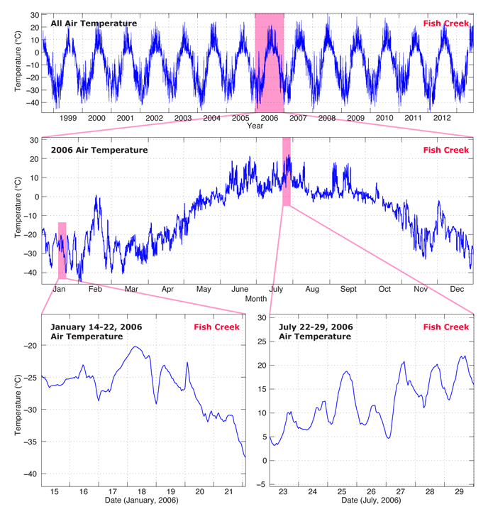
Figure 3. Sample air temperature record from Fish Creek station. Data are presented at several resolutions with each highlighted section expanded. The top panel shows the full record for the station, the middle panel shows 1 full year (2006), the lower left panel shows 1 week during the winter of 2006, and the lower right panel shows 1 week during the summer of 2006.
Figure 4 shows the wind speed record from Fish Creek at hourly resolution. The top panel shows the full record, whereas the middle panel shows 1 full year, and the lower panels show 1 week of winter data and 1 week of summer data. Seasonal patterns are evident with the strongest wind events occurring during winter and the most consistent wind speeds occurring during the summer. The strongest winds, which are related to passing weather systems, are about 20 m s-1 at this site. Occasional gaps in the sub-0 °C portion of the record (upper and middle panels) are due to significant ice buildup on the wind monitor; the data have been masked during these periods. As with air temperature, passing weather systems are the dominant source of wind speed variability during the winter (lower left panel). A diurnal signal is apparent in the summer wind speed variability (lower right panel).

Figure 4. Sample wind speed record from Fish Creek station. Data are presented at several resolutions with each highlighted section expanded. The top panel shows the full record for the station, the middle panel shows 1 full year (2006), the lower left panel shows 1 week during the winter of 2006, and the lower right panel shows 1 week during the summer of 2006.
Figure 5 shows wind roses at the Fish Creek station for each of the four seasons: winter (December, January, February), spring (March, April, May), summer (June, July, August), and autumn (September, October, November). Wind roses are useful for showing how both wind speeds and directions are distributed at a particular site. For the DOI/GTN-P dataset, wind roses are calculated by dividing the wind direction into 16 categories (22.5° each) and the wind speed into three classes: (a) less than 5 m s-1, (b) between 5 m s-1 and 10 m s-1, and (c) greater than 10 m s-1. The wind roses show that winds at Fish Creek most frequently come out of the east and east-northeast. The strongest winds occur during the winter and tend to come out of the east with a secondary maximum out of the west. Strong winds also occur during the transition seasons, autumn and spring, again primarily coming out of the east with a secondary maximum out of the west.
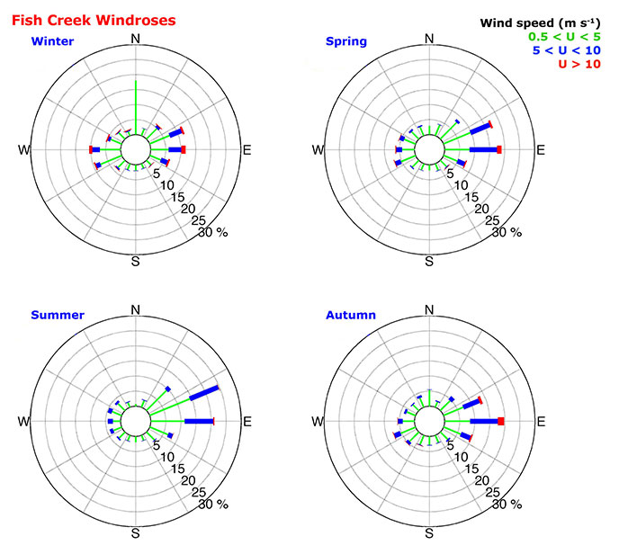
Figure 5. Sample wind roses from Fish Creek station. The wind direction and speed data for a site are divided into 16 wind direction categories (22.5° each) and 3 wind speed classes: (a) less than 5 meters per second (m s–1), (b) between 5 m s-1 and 10 m s-1, and (c) greater than 10 m s-1. The percentage of time that wind speeds occupy each class and directional category (concentric rings) is presented for each season: winter (December, January, February), spring (March, April, May), summer (June, July, August), and autumn (September, October, November). U, wind speed; N, north; E, east; S, south; W, west)
Figure 6 shows the ground temperature record from the Fish Creek monitoring station at hourly resolution. The top panel shows the full record, the middle panel shows a single year of data, and the lower panels show 1 week of winter data and 1 week of summer data. The annual seasonal cycle is clearly evident in the top panel with minimum winter ground temperatures near the surface (5 cm) dropping to about –20 °C and –15 °C at depth (120 cm). Maximum summer temperatures near the surface (5 cm) reach +10 °C and –2 °C at depth (120 cm). In the middle panel, seasonal changes are clearly evident with fast warming in the spring when snow melts and the low-albedo tundra surface is able to absorb shortwave radiation. In the autumn, the water-saturated soils take a long time to freeze solid due to the release of latent heat. In addition to the seasonal cycle, temperature excursions due to passing weather systems are discernible in the middle panel. These weather systems, as well as variability in snow cover, are the dominant source of ground temperature variability during the winter (lower left panel). During the summer, ground temperature variations in the active layer (0–25 cm at Fish Creek) are primarily related to changes in the incident solar flux, which produces a strong diurnal cycle (lower right panel). Ground temperatures below the active layer in summer are reflective of longer term (annual) conditions including air temperature and previous winter snow cover.
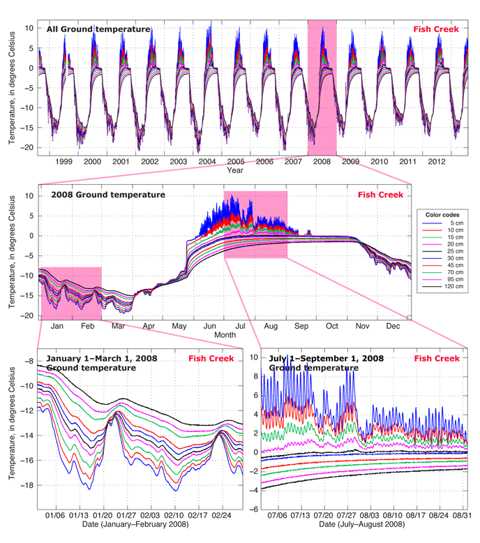
Figure 6. Sample ground temperature record from Fish Creek station. Data are presented at several resolutions with each highlighted section expanded. The top panel shows the full record for the station, the middle panel shows 1 full year (2008), the lower left panel shows 2 months during the winter of 2008, and the lower right panel shows 2 months during the summer of 2008. Cm, centimeter.
Figure 7 shows the incident solar flux from the Fish Creek monitoring station at hourly resolution. The top panel shows the full record; the bottom panel shows a single year of data. The annual seasonal cycle is clearly evident with maximum flux values in mid-summer of about 600 to 700 watts per meter squared and values that drop to zero for about 2 months of winter. Cloudy periods are often evident in the peak summer months, June, July, and August, when temperatures are above freezing and sea ice in the adjacent ocean is far offshore providing a consistent moisture source for cloud formation.

Figure 7. Sample incident solar-flux record from Fish Creek station. Data are presented at two resolutions with one highlighted section expanded. The top panel shows the full record for the station; the bottom panel shows 1 full year (2007).
Figure 8 shows the reflected shortwave radiation flux from the Fish Creek monitoring station at hourly resolution. The top panel shows the full record; the bottom panel shows a single year of data. The annual seasonal cycle is clearly evident with maximum flux values in mid-spring of about 600 watts per meter squared and values that drop to zero for about 2 months of winter. A distinguishing feature of the reflected solar-flux data is the extremely rapid decrease in values during snowpack disintegration. This transition from snow cover to bare tundra usually occurs in late May or early June, and in the span of 5–7 days reflected solar-flux values drop from 600 to 150 watts per meter squared.
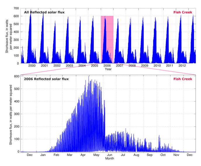
Figure 8. Sample reflected solar-flux record from Fish Creek station. Data are presented at two resolutions with one highlighted section expanded. The top panel shows the full record for the station; the bottom panel shows 1 full year (2006).
Figure 9 shows the entire accumulated rainfall record from the Inigok monitoring station (lat 69°59.377'N., long 153°05.630'W.) at four different resolutions: seasonal (top left panel), monthly (top right panel), weekly (bottom left panel), and daily (bottom right panel). The rainfall season typically begins in early June and ends in late September to early October, with the greatest rainfall amounts occurring in August.
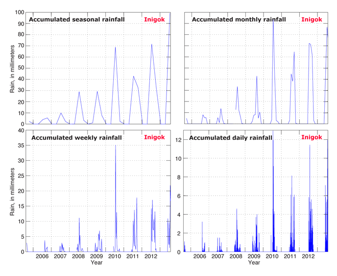
Figure 9. Sample rainfall record from Inigok station. Data are presented at several resolutions. The top left panel shows the accumulated rainfall at seasonal resolution. The top right panel shows the accumulated rainfall at monthly resolution. The bottom left panel shows the accumulated rainfall at weekly resolution. The bottom right panel shows the accumulated rainfall at daily resolution.
Figure 10 shows the snow depth record from the Inigok monitoring station. The top panel shows the full record at hourly resolution; the bottom panel shows a single year of data at daily resolution. The annual seasonal cycle is evident with snow accumulation typically beginning in late September to early October and snowmelt occurring in late May to early June. The snowpack gradually increases through the autumn (October–November), sometimes plateauing in the winter (January–March). Common snowpack features include mid-winter wind scour (evident in the lower panel in late January) and early spring (April–May) snow depth increases immediately prior to snowmelt. A consistent aspect of the snowpack in this region is the extremely rapid disintegration that occurs in late May or early June. Once snowmelt ensues, the entire snowpack is usually gone in 7–10 days. Snow depth varies from station to station with a general trend of increasing depths away from the coast as elevation increases from the coast to the Brooks Range (5–785 m).
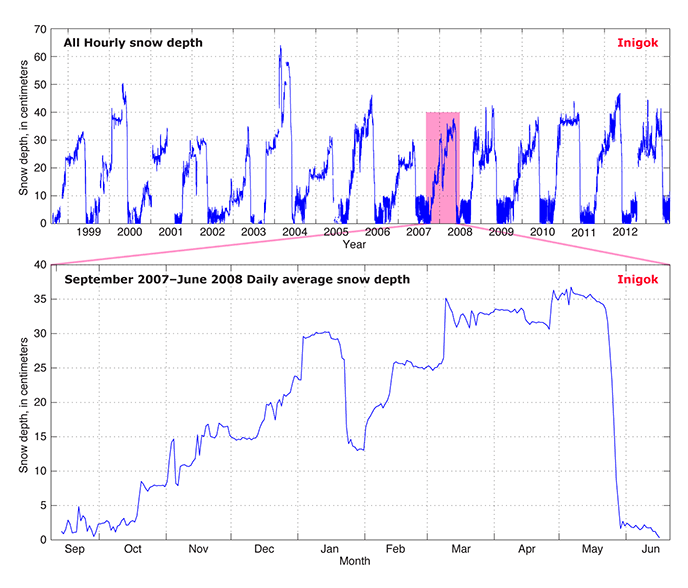
Figure 10. Sample snow depth record from Inigok station. Data are presented at two resolutions with one highlighted section expanded. The top panel shows the full record for the station; the bottom panel shows daily averages for one full snow-cover season, September 2007 through June 2008. Figure 11 shows the hourly resolution soil moisture record at 15-cm depth from the South Meade (lat 70°37.708'N., long 156°50.119'W.) monitoring station. Data gaps in winter occur when the ground temperature falls below about –15 °C, and the sensor does not report valid values. The top panel shows the full record, the bottom panel shows a single year of data, and the inset shows soil-moisture-response details during one summer season. Typical water-fraction values are about 0.4 when the active layer is thawed and near zero when the active layer is frozen. The inset displays a common feature, higher initial water fraction in the soils after snowmelt that gradually dissipates, usually by the end of July. Rains in August and September are often reflected in temporary increases in the water fraction.
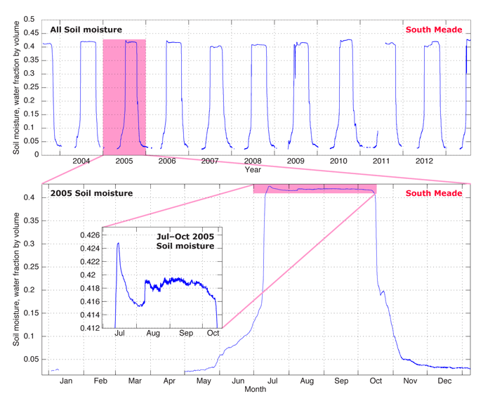
Figure 11. Sample soil moisture record at 15-centimeters depth from South Meade station. Data are presented at several resolutions with each highlighted section expanded. The top panel shows the full record for the station, the bottom panel shows 1 full year (2005), and the inset shows detail during the unfrozen season, July through October, 2005.
Figure 12 shows the surface pressure record from the Fish Creek monitoring station at hourly resolution. The top panel shows the full record; the bottom panel shows a single year of data. A seasonal cycle is evident with fewer high-amplitude pressure changes in spring and summer (late March through mid-October) than in the autumn and winter (November through February).

Figure 12. Sample surface pressure record from Fish Creek station. Data are presented at two resolutions with one highlighted section expanded. The top panel shows the full record for the station; the bottom panel shows 1 full year (2009).
The authors thank and acknowledge all the staff of the Bureau of Land Management (BLM) Arctic Field Office and the U.S. Fish and Wildlife Service (FWS) Fairbanks Field Office whose steady logistical and scientific support has made this ongoing effort possible. In particular, we thank Don Meares, Richard Kemnitz, Shane Walker, Eric Yeager, Connie Adkins, Lon Kelly, and Stacie McIntosh at the BLM, and Janet Jorgenson and David Payer at the FWS. Specific thanks to Jeremy Havens (USGS) for help with manuscript preparation and online publishing. Development of the DOI/GTN-P Observing Network was supported by the U.S. Geological Survey Global Change and Climate History Program (now the Climate and Land Use Change Research and Development Program).
Arctic Council, 2005, Arctic climate impact assessment—Scientific report: Cambridge and New York, Cambridge University Press, 1,046 p.
Chapman, W.L., and Walsh, J.E., 2007, Simulations of Arctic temperature and pressure by global coupled models: Journal of Climate, v. 20, p. 609–632.
Clow, G.D., DeGange, A.R., Derksen, D.V., and Zimmerman, C.E., 2011, Climate change considerations, chap. 4 of Holland-Bartels, Leslie, and Pierce, Brenda, eds., An evaluation of the science needs to inform decisions on Outer Continental Shelf energy development in the Chukchi and Beaufort Seas, Alaska: U.S. Geological Survey Circular 1370, p. 81–108.
DeGange, A., Oakley, K., Irvine, G., Mayfield, G., Frenzel, S., Trawicki, J., Lassuy, D., Woodson, D., Talbot, S., and Wenburg, J., 2005, Future challenges project—Report on the regional workshop for Alaska, Washington, Idaho, and Oregon, June 1–2, 2005, Anchorage, Alaska: U.S. Fish and Wildlife Service and U.S. Geological Survey, 62 p.
Houghton, J.T., Ding, Y., Griggs, D.J., Noguer, M., van der Linden, P.J., Dai, X., Maskell, K., and Johnson, C.A., eds., 2001, Climate Change 2001—The scientific basis—Contribution of Working Group I to the Third Assessment Report of the Intergovernmental Panel on Climate Change: Cambridge and New York, Cambridge University Press, 881 p.
Jeffries, M.O., Richter-Menge, J.A., and Overland, J.E., eds., 2012, Arctic report card 2012: National Oceanic and Atmospheric Administration, Arctic Research Program, accessed September 1, 2012, at http://www.arctic.noaa.gov/reportcard.
Lawrence, D.M., Slater, A.G., Tomas, R.A., Holland, M.M., and Deser, Clara, 2008, Accelerated Arctic land warming and permafrost degradation during rapid sea ice loss: Geophysical Research Letters, v. 35, L11506, doi:10.1029/2008GL033985.
National Research Council, 2001, Climate change science—An analysis of some key questions: National Academies Press, National Research Council–Committee on the Science of Climate Change, 42 p.
National Research Council, 2010, Advancing the science of climate change: National Academies Press, National Research Council–Panel on Advancing the Science of Climate Change, 528 p.
Steinhart, J.S., and Hart, S.R., 1968, Calibration curves for thermistors: Deep-Sea Research, v. 15, p. 497–503.
U.S. Arctic Research Commission, 2003, Climate change, permafrost, and impacts on civil infrastructure: U.S. Arctic Research Commission Permafrost Task Force, Special Report 01–03, 63 p.
Walsh, J.E., 2008, Climate of the arctic marine environment: Ecological Applications, v. 18, no. 2 Supplement, p. S3–S22.
First posted December 10, 2014
For additional information contact:
Director, Geosciences and Environmental Change Science Center
U.S. Geological Survey
Box 25046, Mail Stop 980
Denver, CO 80225
http://gec.cr.usgs.gov/
Part or all of this report is presented in Portable Document Format (PDF). For best results viewing and printing PDF documents, it is recommended that you download the documents to your computer and open them with Adobe Reader. PDF documents opened from your browser may not display or print as intended. Download the latest version of Adobe Reader, free of charge. More information about viewing, downloading, and printing report files can be found here.

![]() U.S. Department of the Interior |
U.S. Geological Survey
U.S. Department of the Interior |
U.S. Geological Survey
URL: http://pubsdata.usgs.gov/pubs/ds/0892/introduction.html
Page Contact Information: GS Pubs Web Contact
Page Last Modified: Monday, 28-Nov-2016 20:30:56 EST

 Abstract