Data Series 258
U.S. GEOLOGICAL SURVEY
Data Series 258
Methods used for the GAMA program were selected to achieve the following objectives: (1) design a sampling plan suitable for statistical analysis, (2) ensure sample collection in a consistent manner, (3) analyze samples using proven and reliable laboratory methods, (4) assure the quality of the ground-water data, and (5) maintain data securely and with relevant documentation.
This study utilized the ground-water basins identified by the DWR (2003) for the study area boundaries (fig. 2). Each of the study areas was subdivided into grid cells approximating 10 mi2 (fig. 7) to provide a spatially unbiased and consistent assessment of ground-water quality (Scott, 1990). For this assessment, the MSSC study area was divided into 21 grid cells, the MSMB study area into 48 grid cells, the MSSV study area into 31 grid cells, and the MSPR study area into 16 grid cells.
Initial target wells (public-supply wells, fig. 7) were obtained from statewide databases maintained by the USGS and the CADHS. If a grid cell contained more than one public-supply well, each well in that grid cell was randomly assigned a rank. In each grid cell with multiple wells, the highest ranked well was given priority for sampling. An attempt was made to select one well per grid cell, but some grid cells did not contain accessible wells. Wells from adjacent cells were selected to substitute for grid cells that had no active wells. In this fashion, a public-supply well was selected for each cell to provide a spatially distributed, randomized monitoring network for each study area. Wells sampled as part of the grid-cell network are referred to, hereafter, as randomized wells.
Additional wells were sampled for the better understanding of a specific topic, including the contribution of aquifers of different depths to water supply (depth-dependent sampling of the monitoring wells), and the source and movement of ground water along the Salinas River (flow-path wells). Wells sampled as part of these studies for better understanding were excluded from the overall statistical characterization of water quality in the MS study unit, as the inclusion of the monitoring and flow-path wells would have caused overrepresentation of certain cells.
Randomized wells sampled as part of the MS study unit were numbered with the following prefixes based on study area: the Santa Cruz study area (MSSC), the Monterey Bay study area (MSMB), the Salinas Valley study area (MSSV), and the Paso Robles study area (MSPR). Additional (nonrandomized) wells were sampled in the Monterey Bay study area to ascertain ground-water quality along flow paths (designated MSMBFP), and at monitoring wells (designated MSMBMW). Randomized wells sampled as part of the MS study unit were numbered with the following prefixes based on study area: the Santa Cruz study area (MSSC), the Monterey Bay study area (MSMB), the Salinas Valley study area (MSSV), and the Paso Robles study area (MSPR). Additional (nonrandomized) wells were sampled in the Monterey Bay study area to ascertain ground-water quality along flow paths (designated MSMBFP), and at monitoring wells (designated MSMBMW).
Table 1 (all tables are shown in back of report) provides the GAMA identification number for each well, along with time and date sampled, sampling schedule, and well-construction information. Ground-water samples were collected from 94 public-supply wells and 3 monitoring wells from July through October 2005. Of the 94 public-supply wells sampled, 51 were in the MSMB study area, 11 in the MSPR study area, 13 in the MSSC study area, and 19 in the MSSV study area. Three monitoring wells located in the MSMB study area also were sampled for the studies for better understanding.
For this study, raw (untreated) ground-water samples were analyzed for 88 VOCs; 122 pesticides and pesticide degradates; 3 constituents of special interest [N-nitrosodimethylamine (NDMA), 1,2,3-trichloropropane (TCP), and perchlorate]; 5 nutrients; dissolved organic carbon (DOC); 10 major and minor ions; 25 trace elements; 12 isotopic constituents; 5 noble gases; alpha and beta radioactivity; and the microbial constituents coliform bacteria and coliphage (tables 2A–2K). General water-quality indicators that were determined in the field were pH, specific conductance (SC), dissolved oxygen (DO), temperature, alkalinity, and turbidity.
Ground-water samples were collected and analyzed for the constituents listed on either the fast, slow, or monitoring-well sampling schedules (table 3). Sixty-three wells were sampled on the fast schedule, 31 wells were sampled on the slow schedule, and 3 wells were sampled on the monitoring-well schedule. All three schedules included the analytes listed on the fast schedule. However, at some wells, additional analytes were added to the fast schedule for special studies for better understanding. For the purposes of this study, this expanded analyte list was named the “slow schedule.” Similarly, at the monitoring wells, additional analytes were added and this schedule was named the “monitoring well schedule.” The fast schedule included analyses for 219 constituents and 2 water-quality indicators, while the slow schedule included analyses of 264 constituents and 6 water-quality indicators. The monitoring well schedule included analyses of 254 constituents and 5 water-quality indicators. In the MS study unit, 65 percent of the ground-water wells were sampled on the fast schedule, 32 percent on the slow schedule, and 3 percent on the monitoring well schedule.
Samples were collected using the USGS National Water-Quality Assessment (NAWQA) program protocols (Koterba and others, 1995; U.S. Geological Survey, 2006). These sampling protocols ensure that a representative sample of ground water was collected at each site and that the samples were collected and handled in a way that minimized the potential for airborne contamination of samples and cross contamination between samples collected at wells. Additional details on sample collection may be found in the analytical method references discussed in the section of this report.
Prior to sampling, each well was pumped continuously to purge at least three casing-volumes of water from the well. Samples were collected from hose-bibs or access points located ahead of points of filtration or chemical treatment, such as chlorination. If a chlorinating system was attached to the well, the chlorinator was shut off at least 24 hours prior to purging and sampling the well to purge the system of extraneous chlorine. For the fast schedule, samples were collected at the well head using a foot-long length of Teflon tubing. For the slow schedule, the samples were collected inside an enclosed flow-through chamber located inside a mobile laboratory and connected to the well head by a 10-50 ft length of the Teflon tubing.
For the field measurements (water-quality indicators), ground water was pumped through a flow-through chamber fitted with a multi-probe meter that simultaneously measures pH, DO, temperature, SC, and turbidity. Measured temperature, pH, DO, and SC values were recorded at 5-minute intervals, for at least 30 minutes, and when these values remained stable for 20 minutes, samples for laboratory analyses were then collected. For analyses requiring filtered water, ground water was diverted through a 0.45-micrometer (μm) vented capsule filter or disk filter. Prior to sample collection, polyethylene sample bottles were pre-rinsed three times using native water. Samples for some constituents were acidified to a pH of 2 or less for preservation. Temperature-sensitive samples were stored on ice prior to daily shipping to the various laboratories. The non-temperature-sensitive samples for tritium, noble gases, chromium speciation, and the isotopic composition of oxygen and hydrogen were shipped monthly, whereas volatile organic compounds, pesticides, compounds of special interest, dissolved organic carbon, radium isotopes, gross alpha and beta radioactivity, and radon-222 samples were shipped daily.
Samples for volatile organic compounds (VOCs), and gasoline additives (table 2A, 2B), and 1,2,3-trichloropropane (1,2,3-TCP) (table 2E) were collected in 40-mL sample vials that were purged with three vial volumes of sample water before bottom-filling to eliminate atmospheric contamination. Six normal (6N) hydrochloric acid (HCl) was added as a preservative to the VOC samples, but not to the gasoline additive samples, nor to the 1,2,3-TCP samples. Pesticides, pesticide degradation products (tables 2C, 2D), and NDMA (table 2E) samples were collected in 1-L baked amber bottles. Pesticide samples were filtered with a glass-fiber filter, whereas the NDMA samples were filtered at the Montgomery Watson-Harza laboratory prior to analysis. Perchlorate (table 2E) samples were collected in 125-mL polyethylene bottles. Nutrient (table 2F) samples were filtered into 125-mL brown polyethylene bottles. DOC (table 2F) samples were collected at the well head after rinsing the sampling equipment with universal blank water. Each ground-water sample for DOC was collected using a 50-mL syringe and 0.45-μm disk filter to filter the water into 125-mL baked glass bottles and then preserved with 4.5 N sulfuric acid.
Ground-water samples for major and minor ions, and trace elements, alkalinity, and total dissolved solids (table 2G) each required filling one 250-mL polyethylene bottle with raw ground water, and one 500-mL and one 250-mL polyethylene bottles with filtered ground water. Each 250-mL filtered sample then was preserved with 7.5 N nitric acid. Mercury (table 2G) samples were collected by filtering ground water into 250-mL glass bottles and preserving each with 6 N HCl. Arsenic and iron speciation (table 2H) samples were each filtered into 250-mL polyethylene bottles that were covered with tape to prevent light exposure, and preserved with 6 N HCl.
Chromium, radon-222, tritium, and dissolved gases were collected from the hose bib at the well head, regardless of the sampling schedule (slow, fast, or monitoring well). Chromium speciation (table 2H) samples were collected using a 10-mL syringe with an attached 0.45-μm disk filter. After the syringe was thoroughly rinsed and filled with ground water, 4 mL were forced through the disk filter, and the next 2 mL of the ground water were filtered slowly into a small centrifuge vial for analysis of total chromium. Hexavalent chromium, Cr (VI), then was collected by attaching a small cation exchange column to the syringe filter, and after conditioning the column with 2 mL of sample water, 2 mL were collected in a second centrifuge vial. Both vials were preserved with 10 μL of 7.5 N nitric acid (Ball and McCleskey, 2003).
Tritium (table 2I) samples were collected at the well head by bottom-filling 1-L polyethylene bottles with unfiltered ground water, after first overfilling the bottles with three volumes of water. Samples for the isotopic composition of oxygen and hydrogen (table 2I) were collected in 60-mL clear glass bottles filled with unfiltered water, sealed with conical caps, and secured with electrical tape to prevent leakage and evaporation. Radium isotopes and gross alpha and beta radiation (table 2I) samples were filtered into 1-L polyethylene bottles and then each acidified with nitric acid. Each carbon isotope (table 2I) sample was filtered before bottom-filling two 500-mL glass bottles that were first overfilled with three bottle volumes of ground water. These samples had no headspace, and were sealed with a conical cap to avoid atmospheric contamination. Samples for alkalinity titrations were collected by filtering ground water into 500-mL polyethylene bottles.
For the collection of radon-222 (table 2I), a stainless steel and Teflon valve assembly was attached to the hose bib at the well head. The valve was closed partially to create back pressure, and a 10-mL sample was taken through a Teflon septum on the value assembly using a glass syringe affixed with a stainless-steel needle. The sample then was injected into a 25-mL vial partially filled with scintillation mixture (mineral oil) and shaken. The vial then was placed in a cardboard tube in order to shield it from light during shipping (U.S. Geological Survey, 2006).
Noble gases (table 2J) were collected in 3/8-in. copper tubes using reinforced nylon tubing connected to the hose bib at the wellhead. Ground water was flushed through the tubing to dislodge any bubbles before flow was restricted with a back-pressure valve. Clamps on either side of the copper tube then were tightened, trapping a sample of ground water for analyses of noble gases (Weiss, 1968).
Microbial constituents also were collected at the well head (table 2K). Prior to the collection of samples, the sampling port was sterilized using isopropyl alcohol, and ground water was run through the sampling port for at least 3 minutes to remove any traces of the sterilizing agent. Two sterilized 250-mL bottles then were filled with ground water for coliform bacteria analyses (total and Escherichia coliform determinations), and one sterilized 3-L carboy was filled for coliphage analyses (F-specific and somatic-coliphage determinations).
Table 4 lists the analytes, the method(s) used for analysis, the laboratory that performed the analyses, and the citations that describe the methods in detail. Nine laboratories performed chemical and microbial analyses for the MS study (see table 4).
In addition to the analytes and their corresponding laboratory methods listed in table 4, selected analyses were done in the field. Alkalinity and the concentrations of bicarbonate (HCO3-) and carbonate (CO32-) were measured by USGS technicians on filtered samples using the Gran titration method (U.S. Geological Survey, 2006). Turbidity, pH, SC, and temperature were measured in the field with calibrated instruments. Dissolved solids were determined by weighing the sample residue on evaporation at 180°C (Fishman and Friedman, 1989). Total coliform bacteria and Escherichia coliform (E. coli) were counted, following a 22–24-hour incubation time, under an ultraviolet light.
Data reporting for the GAMA program addresses two important issues beyond simply presenting the concentrations of the constituents detected. First, it is important to document each laboratory’s capability to either detect an analyte, or to report its absence with confidence. This documentation includes the laboratory reporting levels and detection limits for each analyte (tables 2A–2K), and is explained in the Laboratory Reporting Levels and Detection Limits section. Second, for analytes that were analyzed using more than one method, it is important to know which method is the preferred method; to accomplish this, we present reporting conventions for constituents on multiple analytical schedules in the Constituents on Multiple Analytical Schedules section.
The isotopic composition of oxygen and hydrogen of a sample are expressed in standard delta (δ) notation, in units of permil (parts per thousand), as the differences relative to Standard Mean Ocean Water (SMOW) (Craig, 1961). For example,
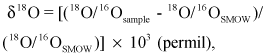
and
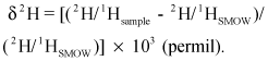
By convention the value of SMOW is 0 per mil.
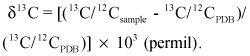
Carbon-13 abundance is expressed by means of the standard δ13C parameter, in units of per mil, which is the difference in the carbon-13/carbon-12 ratio relative to University of Chicago Peedee Formation Standard (PDB) (Friedman and O’Neil, 1977). For example,
The concentration of tritium (hydrogen-3) is measured in picocuries per liter of water (pCi/L). A picocurie per liter represents 2.22 disintegrations of hydrogen-3 per minute per liter of water.
The USGS NWQL uses the laboratory reporting level (LRL) as a threshold for reporting analytical results. The LRL is set to minimize the reporting of false negatives (not detecting a compound when it actually is present in a sample) to less than 1 percent (Childress and others, 1999). The LRL is set at two times the long-term method detection level (LT-MDL), which is the average method detection limit calculated from multiple analytical measurements (>50) of low-level standard solutions. The method detection limit is the minimum concentration of a substance that can be measured and reported with 99-percent confidence that the concentration is greater than zero (at the method detection limit, there is a less than 1 percent chance of a false positive) (U.S. Environmental Protection Agency, 2002a).
Detections below the LRL are reported as estimated concentrations (designated with an “E” before the value in the tables and text). For information-rich methods (including the VOC method used in this study), detections below LT-MDL also are reported as E-coded values. E-coded values also result from detections outside the range of calibration for detections that did not pass laboratory quality-control criteria, and for samples that were diluted prior to analysis.
Some concentrations in this study are reported using minimum reporting levels (MRLs) or method uncertainties. The MRL is the smallest measurable concentration of a constituent that may be reported reliably using a given analytical method (Timme, 1995). The method uncertainty generally indicates the precision of a particular analytical measurement; it gives a range of values wherein the true value will be found.
The reporting levels for selected radioactive constituents (gross-alpha radioactivity, gross-beta radioactivity, radium-226, and radium-228) are based on a sample-specific minimum detectable concentration (SSMDC), a critical value (also sample specific), and the combined standard uncertainty (CSU) (U.S. Environmental Protection Agency and others, 2004). In this report, a result above the critical value represents a greater-than-95-percent certainty that the result is greater than zero (significantly different from the instruments background response to a blank sample), whereas a result above the SSMDC represents a greater-than-95-percent certainty that the result is greater than the critical value (U.S. Environmental Protection Agency and others, 2004). Using these reporting level elements, three unique cases were possible when screening the raw analytical data. First, if the analytical result is less than the critical value (case 1), the analyte is considered not detected, and a value is presented in the table as less than the SSMDC. If the analytical result is greater than the critical value, the ratio of the CSU to the analytical result (relative CSU) was calculated as a percent. For those samples with results that have a relative CSU less than 20 percent, the analytical result is reported unqualified (case 2). For those samples with results that have a relative CSU greater than 20 percent, the analytical results were qualified as estimated values and are preceded in the table with an “E” (case 3). For table clarity, only the screened results are reported here.
Fourteen constituents targeted in the MS study were measured on more than one analytical schedule, or at more than one laboratory (table 5). Results from certain analytical schedules are preferred over others because the methodology is more accurate or precise, and generally yields a greater sensitivity for a given compound. The preferred method for USGS laboratories was selected by the laboratory on the basis of detection levels (http://wwwnwql.cr.usgs.gov/USGS/Preferred_method_selection_procedure.html). If a VOC, gasoline additive, pesticide, or pesticide degradate appears on multiple USGS analytical schedules, then only the measurement determined by the preferred analytical schedule is reported.
Five constituents also were analyzed by more than one laboratory, in which case both results are reported. The VOC 1,2,3-trichloropropane was analyzed at both the NWQL and at the Montgomery Watson-Harza laboratory (MWH). Since the MWH laboratory had a lower reporting level (0.005 µg/L), it was the preferred method for this constituent. Ground-water samples for arsenic, chromium, and iron also were analyzed at two different laboratories; total concentrations were measured at the NWQL in Denver, Colorado, while elemental speciation was measured at the USGS National Research Program (NRP) laboratory in Boulder, Colorado. For arsenic, chromium, and iron, the standard analytical techniques were preferred to the research laboratory methods.
Quality-control (QC) samples collected in the MS study include source-solution blanks, field blanks, replicates, matrix spikes, and surrogates. QC samples were collected to evaluate bias and variability of the water-quality data that may have resulted from sample collection, processing, storage, transportation, and laboratory analysis. The data handling protocols, and the quality control design and assessment that the USGS field members and laboratories utilized, follow the Quality Assurance plan of the National Water Quality Laboratory (Maloney, 2005).
Blank samples (blanks) were collected using nitrogen-purged pesticide-grade “Universal” blank water that was certified to contain less than the LRL or MRL of the analytes investigated in the study. Two types of blanks were collected: source-solution blanks, and field blanks. Source-solution blanks were collected to verify that the blank water used for the field blanks was free of analytes. Source-solution blanks and field blanks were collected at 12 percent of the wells sampled, to determine if equipment or procedures used in the field or laboratory introduced contamination.
Source-solution blanks were collected at the sampling site by pouring blank water directly into sample containers that were preserved, stored, shipped, and analyzed in the same manner as the ground-water samples. For field blanks, blank water was either pumped or poured through the sampling equipment (fittings and tubing) used to collect ground water, then processed and transported using the same protocols as for the ground-water samples. Field blanks were analyzed for VOCs, pesticides, nutrients, dissolved organic carbon, major and minor ions, trace elements, and the microbial constituents.
If a constituent was detected in a field blank, the associated source-solution blank results were examined for similar constituent detections. If the field blank and the source-solution blank contained the constituent, then the source-solution water was interpreted as the origin of the contamination in the blanks, and the field-blank detections using the same blank water were disregarded. If a field-blank detection could not be attributed to the source solution, then the ground-water samples collected prior to and following the collection of the blank were evaluated. If the ground-water samples prior to or following the collection of the contaminated field blank had no detections, then carry-over contamination was ruled out. If an analyte was detected in a blank at a concentration greater than the concentration measured in a ground-water sample collected prior to or following the blank sample, then that ground-water value was censored (table 6). Censored values are indicated by a ‘V’ or ‘VE’ preceding the value in the tables, and were not considered in the summary statistics. If a compound was detected in multiple field blanks, and the detections could not be attributed to the source-solution water, then any ground-water sample that had a detection of that compound in question was evaluated for possible contamination and censored if necessary.
Sequential replicate samples (replicates) were collected to assess variability that may result from the processing and analyses of inorganic and organic constituents. Relative standard deviation (RSD) of the measured values was used to determine the variability within replicate pairs for each constituent (table 7). The RSD is defined as the standard deviation of the replicate pair, divided by the mean concentration for each replicate pair of samples, multiplied by 100, with the result expressed as a percentage. If one value in a sample pair was reported as a nondetection, and the other value was reported as an estimated value below the LRL or MRL, the RSD was set to zero because the values are analytically identical. If one value in a sample pair was reported as a nondetection and the other value was greater than the LRL or MRL, then the nondetection value was set equal to one-quarter of the LRL (Childress and others, 1999) and the RSD was calculated. High RSD values for replicates with low concentrations may indicate higher analytical uncertainty, particularly for concentrations within an order of magnitude of LT-MDL or MDL.
Addition of a known concentration of a constituent (‘spike’) to a replicate environmental sample enables the analyzing laboratory to determine the effect of the matrix, in this case ground water, on the analytical technique used to measure the constituent. The constituents added (matrix spikes) are the same as those being analyzed in the method. This addition enables an analysis of matrix interferences on a compound-by-compound basis. The following matrix spikes were added to 10 percent of the samples in the MS study: VOCs, gasoline additives, pesticides, and pesticide degradates, at the laboratory performing the analysis. Compounds with low recoveries (<70 percent) are of potential concern if environmental concentrations are close to the MCLs; a concentration below an MCL could be falsely indicated (tables 8A, 8B). Conversely, compounds with high recoveries (>130 percent) are of potential concern if the environmental concentrations exceed MCLs: a high recovery could falsely indicate a concentration above the MCL. Recoveries between 70 to 130 percent for matrix spikes were considered acceptable in this study (Fishman and Friedman, 1989).
Surrogate compounds (surrogates) are added to environmental samples in the laboratory prior to analyses in order to evaluate the recovery of similar constituents. Surrogate compounds were added to all ground-water and quality-control samples that were analyzed for VOCs, gasoline additives, pesticides, pesticide degradates, and constituents of special interest. The compounds selected for use as surrogates normally are not found in environmental samples and are used to identify potential problems associated with laboratory analyses. Potential problems include matrix interferences (such as high levels of dissolved organic carbon) that produce a positive bias, and (or) incomplete laboratory recovery (possibly due to improper maintenance and calibration of analytical equipment) that produces a negative bias. Surrogates are used to identify general problems that may arise during sample analysis that could affect the analytical results for all compounds, whereas matrix spikes are used to indicate problems with specific compound analysis. A 70-130 percent recovery of surrogates generally is considered acceptable; values outside this range indicate possible problems with the processing and analysis of samples (table 9) (Connor and others, 1998; Sandstrom and others, 2001).

![]() U.S.
Department of the Interior | U.S. Geological
Survey
U.S.
Department of the Interior | U.S. Geological
Survey
Persistent URL: https://pubs.water.usgs.gov/ds258/
Page Contact Information: Publications Team
Page Last Modified: Monday, 28-Nov-2016 12:29:02 EST
