Seafloor character--Offshore of San Francisco, California

Metadata also available as - [Outline] - [Parseable text] - [XML]

Frequently anticipated questions:


What does this data set describe?

Title: Seafloor character--Offshore of San Francisco, California
Abstract:
This part of DS 781 presents the seafloor-character map (see sheet 5) Offshore of San Francisco, California (raster data file is included in "SFC_OffshoreSanFrancisco.zip," which is accessible from <https://pubs.usgs.gov/ds/781/OffshoreSanFrancisco/data_catalog_OffshoreSanFrancisco.html>). This raster-format seafloor-character map shows six substrate classes of Offshore of San Francisco, California. The substrate classes mapped in this area have been further divided into the following California Marine Life Protection Act depth zones and slope classes: Depth Zone 2 (intertidal to 30 m), Depth Zone 3 (30 to 100 m), Depth Zone 4 (100 to 200 m), Slope Class 1 (0 degrees - 5 degrees), and Slope Class 2 (5 degrees - 30 degrees). Depth Zone 1 (intertidal), Depth Zone 5 (greater than 200 m), and Slopes Classes 3-4 (greater than 30 degrees) are not present in the region covered by this block. The map is created using a supervised classification method described by Cochrane (2008), available at <http://doc.nprb.org/web/research/research%20pubs/615_habitat_mapping_workshop/Individual%20Chapters%20High-Res/Ch13%20Cochrane.pdf>.
References Cited:
California Department of Fish and Game, 2008, California Marine Life Protection Act master plan for marine protected areas; Revised draft: California Department of Fish and Game, accessed April 5 2011, at <http://www.dfg.ca.gov/mlpa/masterplan.asp>.
Cochrane, G.R., 2008, Video-supervised classification of sonar data for mapping seafloor habitat, in Reynolds, J.R., and Greene, H.G., eds., Marine habitat mapping technology for Alaska: Fairbanks, University of Alaska, Alaska Sea Grant College Program, p. 185-194, accessed April 5, 2011, at <http://doc.nprb.org/web/research/research%20pubs/615_habitat_mapping_workshop/Individual%20Chapters%20High-Res/Ch13%20Cochrane.pdf>.
Sappington, J.M., Longshore, K.M., and Thompson, D.B., 2007, Quantifying landscape ruggedness for animal habitat analysis--A case study using bighorn sheep in the Mojave Desert: Journal of Wildlife Management, v. 71, p. 1419-1426.
  1. How should this data set be cited?

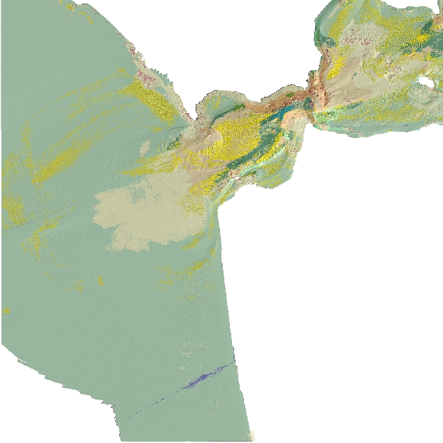
    Erdey, Mercedes D., and Cochrane, Guy R., 2014, Seafloor character--Offshore of San Francisco, California:.

    This is part of the following larger work.

    Cochrane, Guy R., Johnson, Samuel Y., Dartnell, Peter, Greene, H. Gary, Erdey, Mercedes D., Golden, Nadine E., Hartwell, Stephen R., Endris, Charles A., Mansion, Michael W., Sliter, Ray W., Kvitek, Rikk G., Watt, Janet T., Ross, Stephanie L., and Bruns, Terry R., 2015, California State Waters Map Series--Offshore of San Francisco Map Area, California: Open-File Report OFR 2015-1068, U.S. Geological Survey, Reston, VA.

    Online Links:

  2. What geographic area does the data set cover?

    West_Bounding_Coordinate: -122.785224
    East_Bounding_Coordinate: -122.415053
    North_Bounding_Coordinate: 37.939818
    South_Bounding_Coordinate: 37.696678

  3. What does it look like?

    <https://pubs.usgs.gov/ds/781/OffshoreSanFrancisco/images/SeafloorCharacter_OffshoreSanFrancisco.jpg> (JPEG)
    Seafloor character types offshore San Francisco.

  4. Does the data set describe conditions during a particular time period?

    Beginning_Date: 2004
    Ending_Date: 2008
    Currentness_Reference: ground condition

  5. What is the general form of this data set?

    Geospatial_Data_Presentation_Form: GeoTiff

  6. How does the data set represent geographic features?

    1. How are geographic features stored in the data set?

      This is a Raster data set. It contains the following raster data types:

      • Dimensions 8951 x 7939 x 1, type Pixel

    2. What coordinate system is used to represent geographic features?

      The map projection used is WGS 1984 UTM Zone 10N.

      Projection parameters:
      Scale_Factor_at_Central_Meridian: 0.9996
      Longitude_of_Central_Meridian: -123.0
      Latitude_of_Projection_Origin: 0.0
      False_Easting: 500000.0
      False_Northing: 0.0

      Planar coordinates are encoded using coordinate pair
      Abscissae (x-coordinates) are specified to the nearest 2.0
      Ordinates (y-coordinates) are specified to the nearest 2.0
      Planar coordinates are specified in Meter

      The horizontal datum used is D WGS 1984.
      The ellipsoid used is WGS 1984.
      The semi-major axis of the ellipsoid used is 6378137.0.
      The flattening of the ellipsoid used is 1/298.257223563.

  7. How does the data set describe geographic features?

    SeafloorCharacter_OffshoreSanFrancisco.tif.vat
    The shapefile attributes include VALUE - code for the seafloor character classes, COUNT - number of pixels, SLOPE - slope classes, DEPTH_ZONE - depth zones, SUBSTRATE - substrate classes, SUBST_DESC - short description of substrate classes, and FULL_DESC - detailed description of substrate classes. The shapefile can be added to any ESRI ArcMap project. (Source: ESRI)

    Rowid
    Internal feature number. (Source: ESRI)

    Sequential unique whole numbers that are automatically generated.

    VALUE
    This seafloor-character class was produced using video-supervised maximum-likelihood classification of the bathymetry and backscatter (intensity of return) signals from sonar systems. Derivative roughness (rugosity) and backscatter intensity were used as variants in the classification. The resulting four substrate classes (1-4) were divided into the Depth Zones (see Attribute: DEPTH_ZONE) by adding to the original grid value in increments of 10. Depth Zone 2, add 0 to grid value; Depth Zone 3, add 10 to grid value; Depth Zone 4, add 20 to grid value; and Depth Zone 5, add 30 to grid value. The resulting grid was further classified into Slope Classes (see Attribute: SLOPE) by adding to the classified raster values (including depth zones) in increments of 50. Slope Class 1, add 0 to grid value; Slope Class 2, add 50 to grid value; Slope Class 3, add 100 to grid value; and Slope Class 4, add 150 to grid value. (Source: ESRI)

    Range of values
    Minimum:1
    Maximum:74
    Units:Integers 1 - 74 representing seafloor character classes.

    COUNT
    The number of pixels (2m x 2m size grid cell) represented in each seafloor class (see Attribute: VALUE). (Source: ESRI)

    Range of values
    Minimum:1244
    Maximum:29330143
    Units:Integers 1244 - 29330143 pixel count.

    SLOPE
    The slope zones for the final seafloor-character map grid were identified on the basis of the smoothed bathymetry grid. The smoothing was done by applying focal statistics to the original bathymetry grid. The tool uses a moving window and calculates the mean value of the central pixel within a circular neighborhood of 20 m radius along the whole raster map. The resulting raster map represents a smoothed value highlighting overall trends and eliminates local varieties in the terrain (such as higher slopes along rock outcrops). Slope class values are: 1 (flat; 0 degrees to 5 degrees), 2 (sloping; 5 degrees to 30 degrees), 3 (steeply sloping; 30 degrees to 60 degrees), or 4 (vertical; 60 degrees to 90 degrees), or 5 (overhang; greater than 90 degrees). (Source: USGS)

    Range of values
    Minimum:1
    Maximum:2
    Units:Integer value 1 and 2 representing slope classes as described above.

    DEPTH_ZONE
    The depth zones for the final seafloor-character map grid were identified on the basis of the smoothed bathymetry grid. The smoothing was done by applying focal statistics to the original bathymetry grid. The tool uses a moving window and calculates the mean value of the central pixel within a circular neighborhood of 20 m radius along the whole raster map. The resulting raster map represents a smoothed value highlighting overall trends and eliminates local varieties in the terrain (such as varying depths along rock outcrops). Depth Zone values are: Depth Zone 1, intertidal; Depth Zone 2, intertidal to 30 m; Depth Zone 3, 30 to 100 m; Depth Zone 4, 100 to 200 m; and Depth Zone 5, deeper than 200 m (California Department of Fish and Game, 2008). (Source: USGS)

    Range of values
    Minimum:2
    Maximum:4
    Units:Integer values 2-4 representing slope classes as described above.

    SUBSTRATE
    Coded values of the substrate classes. Class 1, Fine- to medium-grained smooth sediment; Class 2, Mixed smooth sediment and rock; Class 3, Rock and boulder, rugose; Class 4, Medium- to coarse- grained sediment; Class 5, Smooth, hard anthropogenic material; Class 6, Rugged anthropogenic material (Source: USGS)

    Range of values
    Minimum:1
    Maximum:6
    Units:Integer values 1-6 representing substrate classes as described above.

    SUBST_DESC
    Summary description of the four substrate classes coded by the attribute SUBSTRATE. Class 1, Fine- to medium-grained smooth sediment; Class 2, Mixed smooth sediment and rock; Class 3, Rock and boulder, rugose; Class 4, Medium to coarse grained (Mobile Sed Features); Class 5, Smooth, hard anthropogenic material; Class 6, Rugged anthropogenic material (Source: USGS)

    Names are in text form, maximum length: 50

    FULL_DESC
    Detailed description of the four substrate classes coded by the attribute SUBSTRATE. Class 1, Low backscatter, low rugosity, typically mud to medium-grained sand, often rippled and/or burrowed; Class 2, Moderate to very high backscatter, low rugosity, typically coarse-grained sand, gravel, cobble and bedrock; Class 3, High backscatter, and high rugosity, typically boulder and rugose bedrock; Class 4, Very high backscatter, low rugosity; typically medium- to coarse-grained, rippled sediment with some shell hash in shallow depressions; Class 5, High backscatter and low rugosity; related to development by humans; Class 6, High backscatter and high rugosity; related to development by humans (Source: USGS)

    Names are in text form, maximum length: 250


Who produced the data set?

  1. Who are the originators of the data set? (may include formal authors, digital compilers, and editors)

  2. Who also contributed to the data set?

  3. To whom should users address questions about the data?

    Guy Cochrane
    U.S. Geological Survey, Pacific Coastal and Marine Science Center
    Geophysicist
    400 Natural Bridges Dr.
    Santa Cruz, CA 95060-5792
    USA

    (831)460-7554 (voice)
    (831)427-4709 (FAX)
    gcochrane@usgs.gov


Why was the data set created?

These data are intended for science researchers, students, policy makers, and the general public. These data can be used with geographic information systems or other software to identify local seafloor character.


How was the data set created?

  1. From what previous works were the data drawn?

  2. How were the data generated, processed, and modified?

    Date: Oct-2009 (process 1 of 1)
    The seafloor-character map was produced using video-supervised maximum likelihood classification of the bathymetry and intensity of return from sonar systems. The classification was supervised using signatures defined by hand-drawn polygons located through sediment samples and video-observation ground truthing applying methodology described in Cochrane (2008), available at <http://doc.nprb.org/web/research/research%20pubs/615_habitat_mapping_workshop/Individual%20Chapters%20High-Res/Ch13%20Cochrane.pdf>. The two variants used in this classification were backscatter intensity and derivative rugosity. Rugosity measures terrain ruggedness as the variation in three-dimensional orientation of grid cells within a neighborhood. Vector analysis is used to calculate the dispersion of vectors normal (orthogonal) to grid cells within the specified neighborhood. This method effectively captures variability in slope and aspect into a single measure. Ruggedness values in the output raster map can range from 0 (no terrain variation) to 1 (complete terrain variation). The calculation was performed using the Terrain Ruggedness (VRM) tool (for details, see Sappington and others, 2007).
    Classes I, II and III values were delineated using multivariate analysis. Class IV (mobile sedimentary features) values were determined on the basis of visual characteristics using both bathymetry and backscatter (slight depression in the seafloor, very high backscatter return). Class V and VI classes (smooth and rugged anthropogenic features) were depicted based on visual characteristics and known location of man-made features. The resulting map (gridded at 2 m) was cleaned by hand to remove data-collection artifacts (for example trackline nadir). Editing was performed in Photoshop, with which individual pixels were selected and values adjusted to remove noise. Selection occurred without antialiasing, and the resulting grid was identical but for the edited pixels. The four seafloor classes were then colored to indicate which of the five California MLPA depth zones they are located in: Depth Zone 2 (intertidal to 30 m), Depth Zone 3 (30 to 100 m), Depth Zone 4 (100 to 200 m), or Depth Zone 5 (greater than 200 m). These were further subdivided into one of the following slope classes: Slope Class 1 (0 degrees - 5 degrees), Slope Class 2 (5 degrees - 30 degrees), Slope Class 3 (30 degrees - 60 degrees), or Slope Class 4 (60 degrees - 90 degrees). Depth Zone 1 (intertidal), Depth Zone 5 (greater than 200 m), and Slopes Classes 3-4 (greater than 30 degrees) are not present in the region covered by this block.

  3. What similar or related data should the user be aware of?


How reliable are the data; what problems remain in the data set?

  1. How well have the observations been checked?

    Pixel resolution 2 m.

  2. How accurate are the geographic locations?

    Positional information reflects the position of the camera and was collected using a still photo camera, WAAS-enabled GSP unit, recording at between 1 to 2 nm. DGPS (WAAS) accuracy for position is less than 3 meters. (From Garmin GPSMAP 76C/76CS Specifications, M01-10108-00, Rev0304, <https://buy.garmin.com/shop/store/assets/pdfs/specs/gpsmap76c_76cs_spec.pdf>).

  3. How accurate are the heights or depths?

  4. Where are the gaps in the data? What is missing?

    Total coverage for the survey area is 100%. Survey area is defined by coverage of both the multibeam bathymetry and backscatter datasets.

  5. How consistent are the relationships among the observations, including topology?

    Classification was done on the basis of training samples delineated by interpreter. The classification was performed using mathematical algorithms then hand-edited by the interpreter to remove noise.


How can someone get a copy of the data set?

Are there legal restrictions on access or use of the data?

Access_Constraints: None
Use_Constraints:
Please recognize the U.S. Geological Survey (USGS) and the California State University, Monterey Bay, Seafloor Mapping Lab (CSUMB). USGS-authored or produced data and information are in the public domain. This information is not intended for navigational purposes. Read and fully comprehend the metadata prior to data use. Uses of these data should not violate the spatial resolution of the data.
Where these data are used in combination with other data of different resolution, the resolution of the combined output will be limited by the lowest resolution of all the data. Acknowledge the U.S. Geological Survey in products derived from these data. Share data products developed using these data with the U.S. Geological Survey.
This database has been approved for release and publication by the Director of the USGS. Although this database has been subjected to rigorous review and is substantially complete, the USGS reserves the right to revise the data pursuant to further analysis and review. Furthermore, it is released on condition that neither the USGS nor the United States Government may be held liable for any damages resulting from its authorized or unauthorized use.
Although this Federal Geographic Data Committee-compliant metadata file is intended to document these data in nonproprietary form, as well as in ArcInfo format, this metadata file may include some ArcInfo-specific terminology.


Who wrote the metadata?

Dates:
Last modified: 2013
Last Reviewed: 28-Aug-2014
Metadata author:
Mercedes D. Erdey
U.S. Geological Survey (USGS), Pacific Coastal and Marine Science Center
Geologist
400 Natural Bridges Drive
Santa Cruz, California 95060
USA

(831)460-7416 (voice)
merdey@usgs.gov

Metadata standard:
FGDC Content Standards for Digital Geospatial Metadata (FGDC-STD-001-1998)


Generated by mp version 2.9.16 on Mon May 18 16:09:44 2015