 The Main Shock
| Assisting Recovery | Table of Contents | Geologic Hazards |
The Main Shock
The Northridge earthquake began as a rupture on a hidden fault at a depth of about 17.5 kilometers beneath the San Fernando Valley. For 8 seconds following the initial break, the rupture propagated upward and northwestward along the fault plane at a rate of about 3 kilometers per second. The rupture front spread out across the fault plane, so that the eventual size of the rupture covered an area of approximately 15 by 20 kilometers. The rupture then terminated at a depth of about 5-6 kilometers. Using data from 38 of the more than 200 accelerographs throughout southern California, and data from other instruments and land surveys, scientists were able to make an accurate portrayal of the dynamic properties of the movement along the fault.
| Accelerograms, the recordings from strong-motion accelerographs, contain information about the large-amplitude seismic waves in the region close to large earthquakes. This information is used primarily by engineers to help establish seismic safety codes for future earthquakes. It is also used by seismologists to understand the details of the fault-rupture process and the complicated wave propagation effects that control the intensity of earthquake shaking. |
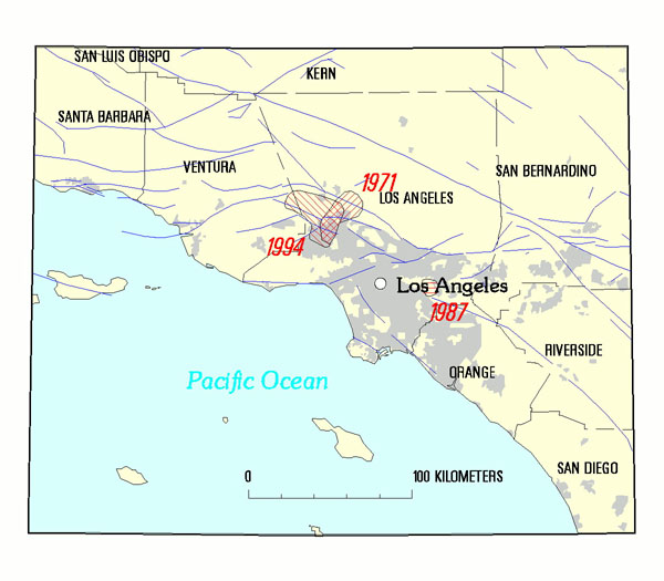 Earthquakes are broad, areal events that move through time and space. The main shock
and aftershock areas of three recent earthquakes in the Los Angeles region show the approximate dimensions of fault
slip beneath the land. Note the overlap of the 1994 Northridge event (M = 6.7) and the 1971 San Fernando event
(M = 6.7). Like the Northridge earthquake, the smaller Whittier Narrows event of 1987 (M = 5.9) occurred on a blind
thrust fault. Principal faults exposed at the surface (purple lines) and urbanized areas of southern California
(gray shaded area) are shown for comparison.
Earthquakes are broad, areal events that move through time and space. The main shock
and aftershock areas of three recent earthquakes in the Los Angeles region show the approximate dimensions of fault
slip beneath the land. Note the overlap of the 1994 Northridge event (M = 6.7) and the 1971 San Fernando event
(M = 6.7). Like the Northridge earthquake, the smaller Whittier Narrows event of 1987 (M = 5.9) occurred on a blind
thrust fault. Principal faults exposed at the surface (purple lines) and urbanized areas of southern California
(gray shaded area) are shown for comparison.
The fault movements were characterized by at least three distinct subevents, or pulses of motion, a few seconds apart. The initial subevent came from an asperity (p. 14) that began at the hypocenter and extended upward (updip). Another large subevent was centered about 12 kilometers updip to the north from the hypocenter. A third subevent radiated from a high-slip region about 19 kilometers deep, 8 kilometers west-northwest of the hypocenter.
The Northridge earthquake exhibited an amplification effect, known as directivity, where the amplitude of the seismic waves was larger in the forward direction of the rupture. Fortuitously, this resulted in the strongest long-period (1-3 second) ground motions accruing in areas north of the San Fernando Valley that were sparsely populated. Also, this region had few larger steel- or concrete-frame structures which are especially vulnerable to energy of periods in the range of 1-3 seconds. Consequently, ground motions in the most populated and built-up areas of the valley to the south were modest relative to those in the Santa Susana Mountains and the Santa Clara River valley.
For engineering design and hazards assessment during the recovery process, scientists estimated ground motions throughout the region to fill in broad areas where no direct instrumental measurements were made (see p.65). Estimates were based on a model developed for the fault-plane rupture, and allowed for analysis of damage potential over the entire near-source region. The estimates took into account, for example, the longer period directivity pulses, while realistically representing higher frequency accelerations needed for engineering design.
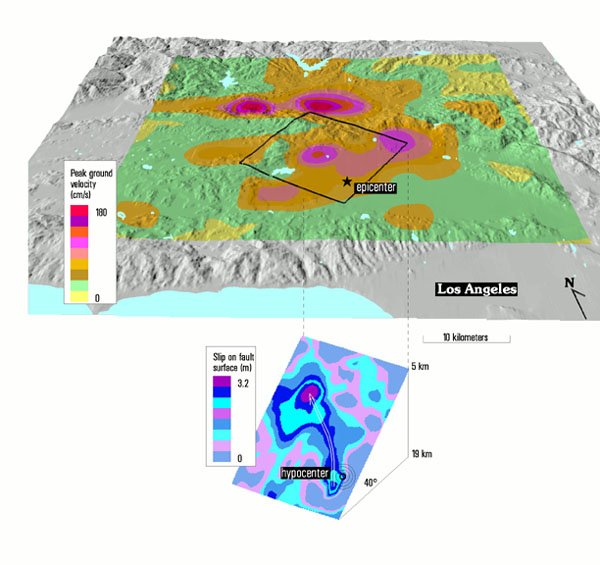
| This perspective aerial view of the Los Angeles region from the south illustrates how the Earth ruptured beneath the San Fernando Valley and shows some of the effects the resulting earthquake had on the land above. |
Effects at the Land Surface
Color tints on the surface show the distribution of peak ground velocities inferred from strong-motion accelerograms. The rectangle is the projected outline of the subsurface fault plane, and the star is the epicenter, the point on the land surface directly above the hypocenter. The highest values of peak ground velocities occurred about 15 kilometers north and west of the epicenter. These high values are thought to be the result of the movement of a block of earth upward and to the northwest, and to the shock being amplified in sedimentary basins.
The Fault Plane
Based on observations of strong ground motions and deformations of the land surface, scientists have portrayed the buried fault plane illustrated here. The fault plane is located between 5 and 19 kilometers beneath the surface. The modeled slip surface is about 430 square kilometers, although the slip did not occur over that entire surface. The plane dips about 40° to the south-southwest. The inferred amounts of slip on the plane are shown by different colors, and the color patterns suggest the progression of movement of the upper block of earth with respect to that below the plane. Maximum slip on the plane, seen in the northwest quadrant, was about 3 meters. Apparently, movement that began at the hypocenter in the southeast quadrant generally proceeded upward and to the northwest (arrow). (Note that the plane is shown displaced well below the surface.)
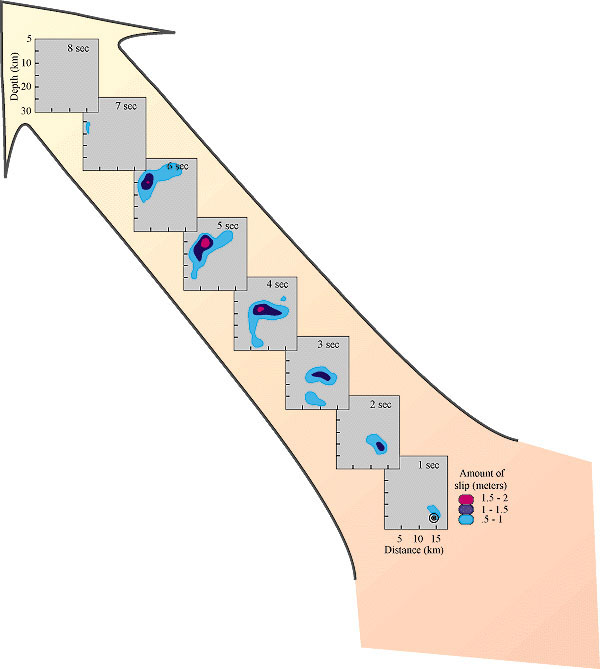 Portraying
the Way the Fault Plane Ruptured
Portraying
the Way the Fault Plane Ruptured
An earthquake is a rupture process that expands from an initial point on a fault plane called the hypocenter. The rupture does not occur instantaneously nor does it proceed uniformly along a fault plane. The Northridge earthquake ruptured the fault plane for about 8 seconds and had an average slip across the plane of about 1 meter. The rupture proceeded across the plane northwesterly from the hypocenter at about 3 kilometers per second. However, some parts of the plane exhibited little or no slip and some parts slipped more than 3 meters. The concentrated areas of larger amounts of slip (at 0-2, 2-3, and 3-5 seconds) are called asperities, which are the sources of pulses of energy that arrive at the surface at different times. Modern seismological techniques allow scientists to model the details of this process to understand its complexity and the broad variety of effects it can cause.
|
The direction in which an earthquake ruptures across its fault plane can greatly affect the intensity of strong ground motion. Depending on its particular fault geometry, another earthquake the same size as the Northridge event could produce even stronger shaking in populated areas of Los Angeles than the shaking experienced in the San Fernando Valley during 1994. |
The Northridge earthquake significantly deformed the Earths crust over an area of about 4,000 square kilometers. In general, the earthquake caused uplift throughout the San Fernando Valley and adjacent mountain areas. The Santa Susana Mountains were pushed up by at least 40 centimeters, based on direct measurements at Oat Mountain, and possibly by as much as 52 centimeters, based on modeling slip on the fault plane. The northern edge of the San Fernando Valley was pushed up less than the mountains, but uplift of more than 20 centimeters was measured in Northridge, and as much as 20-40 centimeters of uplift occurred throughout the northern part of the valley.
Over the region of largest slip on the fault plane (see p. 13), the land surface was pressed into an asymmetric dome-shaped uplift. Here, the largest horizontal movements (up to 22 centimeters) also occurred, with displacements outward from the apex of the dome. Significant shortening at the north-northeast and south-southwest margins of the domed area indicates the net compression between the upper and lower blocks of crust that moved during the earthquake.
USGS scientists measured vertical and horizontal displacements using a total of 534 occupations of 66 survey stations during 92 field sessions. These data were combined with continuously recorded Global Positioning System (GPS) data covering 24 hours on the days of each field session. The data were compared with pre-earthquake data collected within 15 months before the earthquake. The resulting data set is of high quality and potentially high utility in understanding the earthquake. The data quality promises to lead to modeling efforts more advanced than the preliminary modeling used to describe the earthquake source for this report.
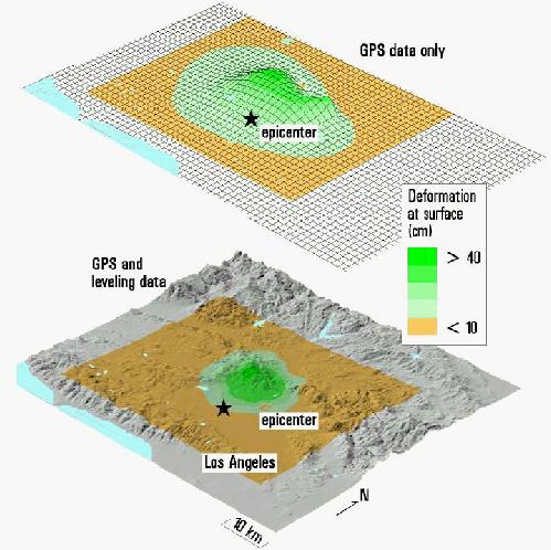
The gentle, roughly symmetrical doming of the Earths surface is a typical result of slip on a deeply buried fault. The diagrams are three-dimensional representations of the section of land uplifted by the earthquake, and clearly illustrate the concept that an earthquake is best considered as a broad area of deformation rather than a point at the epicenter. The upper diagram is a deformation model based only on GPS data. The lower diagram shows the region of uplift computed from GPS and leveling data. The greatest uplift is centered over the northern part of the San Fernando Valley, where the buried, dipping fault plane comes closest to the surface.
| GPS and leveling data and interpretations can be viewed on the WWW at the following Uniform Resource Locator (URL): http://tango.gps.caltech.edu |
Using strong-motion and displacement data, scientists modeled fault geometry and amount of slip. Modeling suggests that a high-slip area occurred updip and northwest of the main shock hypocenter, and that less than 1 meter of slip occurred in the uppermost 5 kilometers of the crust. This finding is consistent with the lack of clear surface rupture, and with the notion that the intersection with the fault that ruptured in the 1971 San Fernando earthquake formed the upper terminus of slip in the Northridge earthquake. Variations in predicting displacements based on the models indicate, however, that the source geometry is more complicated than a single rectangular plane.

Models of the fault planes of the 1994 Northridge (magenta) and 1971 San Fernando earthquakes (blue) suggest that movement on the buried thrust fault responsible for the Northridge earthquake terminated about 5 kilometers beneath the surface. This movement may have terminated against one of the faults that moved in 1971. Stars show positions of the hypocenters of the two shocks, and the arrays of red and blue dots indicate locations of aftershocks. Compare this illustration with the perspective view on page13.
Following the M = 6.7 main shock, thousands of aftershocks occurred in the region of the fault-rupture plane. Aftershocks typically are more numerous immediately following the main shock, and their numbers gradually diminish with time. There were more than 1,000 aftershocks per day during January 1994. By January 1996, aftershocks were still occurring but only at the rate of a few per day. During this period, there were 9 aftershocks in the range M = 5.0-5.9, 42 in the range M = 4.0-4.9, and 353 in the range M = 3.0-3.9. Locations of aftershocks are commonly used as indicators of the areal extent of the earthquake rupture. For the Northridge event, this is shown by the correspondence between the region of aftershocks and the earthquake source areas derived from modeling the fault rupture using strong-motion and geodetic data.
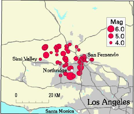 The
aftershock zone of the Northridge earthquake illustrates the broad area affected by movements on the fault plane.
These are some of the largest aftershocks (M >4.0). The largest circle represents the M = 6.7 main shock.
The
aftershock zone of the Northridge earthquake illustrates the broad area affected by movements on the fault plane.
These are some of the largest aftershocks (M >4.0). The largest circle represents the M = 6.7 main shock.
 Lessons
Learned Lessons
LearnedSubsequent work on relocating aftershocks has convinced scientists that the fault geometry is more complicated than either a single uniform-slip dislocation, or distributed slip on a single plane. The rupture almost surely occurred on a more complicated structure that may ultimately be defined by more detailed studies or complex models. The data also suggest that the Northridge earthquake occurred on an eastern extension of the Oak Ridge fault system. There is also a possibility of slip on other faults that might be detected by refinements in modeling. The high-quality seismic and geodetic data will readily lend itself to use in refined models in the future. |
| Geologic Setting | Table of Contents | Geologic Hazards | TOP |
| AccessibilityFOIAPrivacyPolicies and Notices | |
| |
|