Submitted to Proceedings,
5th International Conference on Estuarine
and Coastal Modeling,
M.L. Spaulding and A.F. Blumberg, Eds., ASCE Press
Richard P. Signell
, Harley J. Knebel, Jeffrey H. List and Amy S. Farris Woods Hole Field Center U.S. Geological Survey, Woods Hole, MA, 01543-1598. Tel: (508)-548-8700 E-mail: rsignell@usgs.gov , jlist@usgs.gov, hknebel@usgs.gov,afarris@usgs.gov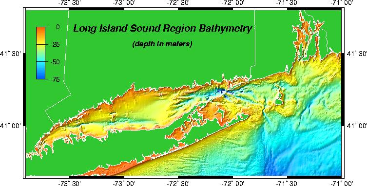
A modeling study was undertaken to simulate the bottom tidal-, wave-, and wind-driven currents in Long Island Sound in order to provide a general physical oceanographic framework for understanding the characteristics and distribution of seafloor sedimentary environments. Tidal currents are important in the funnel-shaped eastern part of the Sound, where a strong gradient of tidal-current speed was found. This current gradient parallels the general westward progression of sedimentary environments from erosion or nondeposition, through bedload transport and sediment sorting, to fine-grained deposition. Wave-driven currents, meanwhile, appear to be important along the shallow margins of the basin, explaining the occurrence of relatively coarse sediments in regions where tidal currents alone are not strong enough to move sediment. Finally, westerly wind events are shown to locally enhance bottom currents along the axial depression of the Sound, providing a possible explanation for the relatively coarse sediments found in the depression despite tide and wave-induced currents below the threshold of sediment movement. The strong correlation between the near-bottom current intensity based on the model results and the sediment response as indicated by the distribution of sedimentary environments provides a framework for predicting the long-term effects of anthropogenic activities.
Long Island Sound is a major east-coast estuary located adjacent to the most densely populated region of the United States. Because of the enormous surrounding population, the Sound has received anthropogenic wastes and contaminants from various sources (Wolfe et al., 1991). As part of its National Coastal and Marine Geology Program, the U.S. Geological Survey is conducting a regional study program designed to understand the processes that distribute sediments and related contaminants in the Sound. Knowledge of the bottom-current regime is crucial both in understanding the distribution of bottom sedimentary environments in the Sound and in predicting the long-term fate of wastes and contaminants which have been introduced there.
There have been numerous observational, theoretical and modeling studies concerning the currents in Long Island Sound. Many of the observational and theoretical studies pertaining to the interaction of bottom currents with the sea floor characteristics are summarized in a series of review papers by Gordon and Bokuniewicz (Gordon, 1980; Bokuniewicz and Gordon, 1980a; Bokuniewicz and Gordon, 1980b; Bokuniewicz, 1980). In these papers, they determine that the character of the seabed is controlled primarily by tidal currents, with a lesser role played by estuarine circulation and storms. Previous modeling studies have explored the M2 tidal response (Kenefick, 1985) and the interaction of estuarine, wind-driven and tidally-driven circulation during a realistic simulation including forcing by observed wind, heat flux, tide and river input (Schmalz, 1993; Schmalz et al, 1994). These studies indicate that the bottom currents in the eastern Sound are dominated by density-driven circulation and tidal residuals, whereas in the central and western Sound other currents are more important than the tidal residuals. In this paper, we use numerical simulations to further define the contribution of three processes that potentially move sediments: tides, wind-waves and storm-induced currents.
|
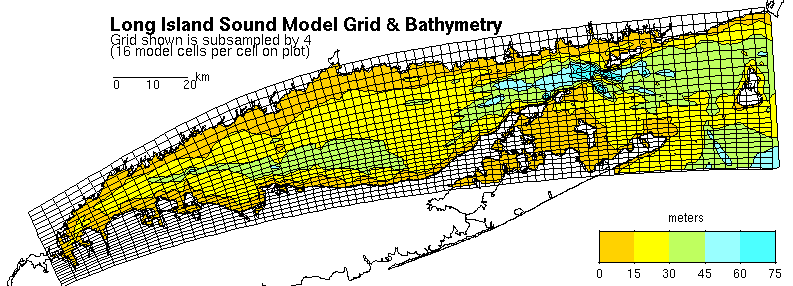
| Figure 1. Long Island Sound model grid and bathymetry. The average depth is 24 m, and the maximum depth exceeds 100 m in the contricted eastern entrance to the Sound. The curvilinear model grid is subsampled by a factor of 4 for clarity. The actual grid cell sizes are between 200 and 400 m. |
Long Island Sound is located between Connecticut and Long Island, New York, on the east
coast of the United States (Figure 1). It is approximately 150 km long, 30 km wide,
and the average water depth is 24 m. A 30-40 m deep axial depression runs east-west
through the western half of the Sound, and water depths reach more than 100 m at the
eastern entrance to the Sound. The Sound opens into the offshore waters of Block Island
Sound on its eastern end (The Race) and is connected to New York Harbor through the East
River on its western end. The system is approximately in quarter-wave resonance with the
semi-diurnal tide, resulting in a threefold increase in tidal range from about 0.8 m on
the eastern end to more than 2.2 m on the western end. Strong tidal currents in excess of
120 cm/s are found at The Race.
Knebel et al. (1997) recently outlined the general distribution of modern seafloor environments in Long Island Sound. They identified four categories of environments based on an extensive regional collection of sidescan sonar data. These categories included: (1) erosion or nondeposition; (2) coarse-grained sediment sorting; (3) sediment sorting and reworking; and (4) fine-grained deposition. In the funnel-shaped eastern part of the Sound, they found a westward progression of bottom environments ranging from erosion or nondeposition at the narrow eastern entrance to the Sound, through an extensive area of bedload transport and sediment sorting, to a region of fine-grained deposition. The broader western Sound, on the other hand, is comprised largely of depositional environments except in local areas of topographic relief where there is a patchy distribution of various other environments. An extensive treatment of the bottom sedimentary environments in Long Island Sound is currently being completed as part of the U.S. Geological Survey regional study program (Knebel et al, 1998, manuscript in preparation). Preliminary analysis indicate that winnowing of sediments occurs along the shallow margins and along some segments of the axial depression of the Sound.
To address the bottom currents associated with tides and strong wind events, we configured a high-resolution model of Long Island Sound capable of representing topography at the 1-2 km scale. We used the Estuary Coastal and Ocean Model (Blumberg and Mellor, 1987) with 10 evenly spaced sigma levels and 300 x 100 grid cells in a curvilinear domain (Figure 1). This resulted in a typical grid spacing of 200-400 m over most of the Sound. The model was run with uniform density because modeling of estuarine circulation was beyond the scope of this study. For open boundary conditions at the eastern, open-ocean end, we specified elevation by M2 tidal constituent data interpolated from Rick Luettich's detailed finite-element tidal model of the East and Gulf Coast (Luettich and Westerink, 1995). For the western end, we specified the M2 amplitude and phase from the NOS tidal data at Willets Point. For the simulations of wind-driven currents, we used a uniform wind stress, and since only tidal heights were specified along the open boundary, the sub-tidal elevation was effectively set to zero. Thus,only the local wind effect was simulated. At the bottom boundary the roughness length z0 was set to 0.67 cm, equivalent to a drag coefficient of Cd= 0.003 at 10 m above the bed. This value of Cd (applied to depth-averaged currents) was found to produce good results in the tidal modeling study of Kenefick (1985). The model was run for 5 tidal cycles, with results saved every 10 lunar minutes over the last cycle. A internal time step of 186.3 seconds was used, with an external time step of 9.31 seconds. The coefficient in the Smagorinsky horizontal viscosity parameterization was set to 0.05.
Tidally-Driven Bottom Currents
As an indicator of the intensity of the bottom currents driven by typical tides, the maximum bottom velocity over the course of the tidal cycle was calculated at 1 m above bottom. The results show strong bottom currents in excess of 50 cm/s in the constricted eastern end of the Sound, but the peak speed decreases westward as the width of the Sound increases (Figure 2). In general, the eastern third of the Sound has bottom tidal speeds between 30 and 60 cm/s, the central third of the Sound has speeds between 20 and 30 cm/s and the western third of the Sound has speeds less than 20 cm/s. Local enhancements of bottom tidal currents exist near headlands and atop cross-Sound shoal complexes in the western Sound; in places the currents exceed 30 cm/s.
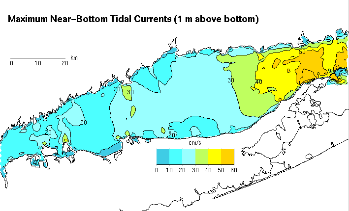 |
| Figure 2. Maximum tidal currents one meter above bottom, driven by M2 tidal
forcing on the open boundaries. |
There is a clear correspondence between the tidal-current distribution and the western
progression of sedimentary environments in the eastern part of the Sound as outlined by
Knebel et al. (1997). Here, areas of erosion or nondeposition, bedload transport, and
sediment sorting occur where the bottom tidal currents exceed about 30 cm/s. These speeds
are consistent with the theoretical calculations of strengths of near-bottom currents
needed to move the sediments that typically compose these environments (fine sand and
coarser) (Knebel et al., 1997). For a bottom roughness of 0.5 cm, the Shields's Curve
velocities required at 1 m above the bottom are 27 cm/s for fine sand (0.125 mm diameter)
and 37 cm/s for coarse sand (0.5 mm diameter) (Butman, 1987).
While the spatial gradients of the strength of the tidal currents explain the general
distribution of sedimentary environments in the eastern Sound, the asymmetry in the
ebb-flood tidal currents can give rise to small-scale residual circulation and
divergence-convergence of bedload transport that can help explain the local maintenance of
selected features in the Sound (Figure 3). Over the Long Sand Shoal, for example, the
tide-induced bottom residual currents indicate clockwise sediment transport and
convergence. This suggests a continuous mechanism for supplying sand to sustain the shoal.
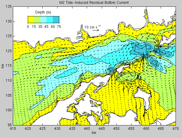 |
| Figure 3. Simulated M2 tide-induced near-bottom (1 m above bottom) residual
currents. |
In addition to tidal currents, the orbital currents associated with waves generated by local winds could be a significant mechanism of bottom sediment resuspension. To better understand the resuspension potential throughout the Sound, we simulated the patterns of bottom orbital currents in the basin with the numerical wave-prediction model, HISWA (HIndcasting Shallow water WAves, Holthuijsen et al., 1989). HISWA computes steady-state wave heights on a rectangular grid over complex topography. It includes the simultaneous effects of wave generation by wind, wave propagation including shoaling and refraction, and wave dissipation through bottom friction and breaking. An incoming wave may be specified as a boundary condition, although this was not used in Long Island Sound because of the nearly fully enclosed nature of the Sound.
A square computational grid was constructed with dimensions 220 x 220 km and grid spacing of 300 m in the wind direction, 600 m perpendicular to the wind direction. This grid was centered on Long Island Sound, allowing prediction of waves generated by wind from all points of the compass. We computed 144 HISWA simulations of the bottom wave orbital velocity maximum, Ub, for winds of 2.5, 5.0, 7.5, 10.0, 12.5, 15.0, 17.5, 20.0 and 22.5 m/s, each at 16 directions equally spaced around the compass.
An example of predicted Ub for winds of 15 m/s from the east-northeast
(typical of a strong winter northeaster) is shown in Figure 4. Under these strong storm
conditions, the significant wave height ranges from 1.5 to 2 m, with typical periods of
4-6 seconds. The bottom velocity ranges from less than 5 cm/s in water deeper than about
20 m to more than 20 cm/s in water shallower than about 10 m, generally found within a few
kilometers of the coast. The wave velocity necessary to resuspend fine-grained muds is
approximately 15 cm/s (Komar and Miller, 1975). Thus wave-induced bottom velocities during
strong wind events could explain the winnowing of sediments observed along the shallow
margins of the Sound.
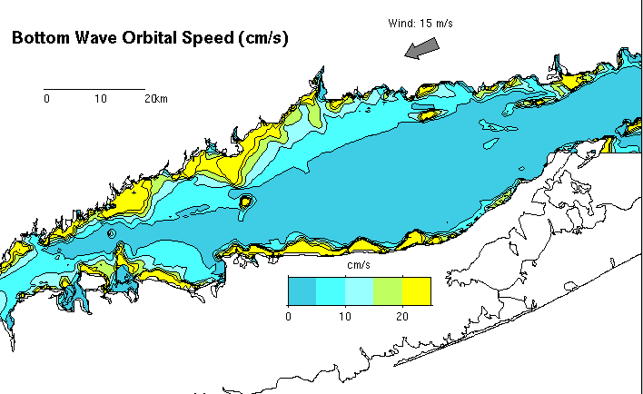 |
| Figure 4. Simulated RMS bottom wave orbital velocities resulting from a 15 m/s
east-northeasterly storm. |
In order to calculate a long-term estimate of Ub throughout the region, the set
of 144 model simulations of bottom orbital velocity were weighted with the wind
distribution over a 12 year period (Nov 1984 - Dec 1996) from the NOAA Ambrose Light
meteorological station. These results are presented as the percentage of time that Ub
is expected to exceed values thought to represent the threshold for the initiation of
sediment resuspension. An example is given in Figure 5 for a threshold of 15 cm/s. Similar
to the northeasterly storm example, the percentage of time that Ub exceeds
threshold values is greatest in a thin strip around the periphery of the Sound, and the
threshold value is exceeded less than 0.001 percent of the time in water depths greater
than about 20 m. This is consistent with estimates of wave influence by Bokuniewicz and
Gordon (1980b).
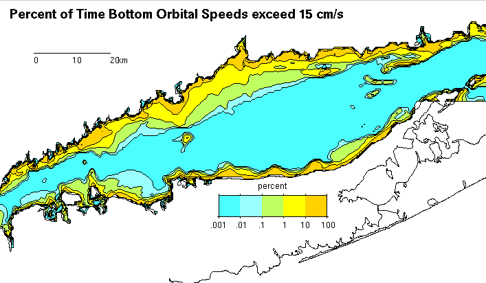 |
| Figure 5. Percentage of time that the RMS bottom wave orbital velocities exceed 15
cm/s, based of 12 years of wind data from the NOAA Ambrose Light meteorological
station. |
In addition to driving surface waves, strong wind events in the Sound generate bottom
currents which may influence the distribution of sedimentary environments. Observations of
low-passed (33 hour) bottom currents and winds show strong correlation at zero lag
(Blumberg, 1997, personal communication); thus it is appropriate to examine the steady
response of the Sound to wind. Similar to the steady wind response in a long lake
(Csanady, 1973), the currents in Long Island Sound respond most efficiently to the
along-axis wind component, and circulation is generally downwind in the shallows and
against the wind in the deeper reaches (Figure 6). A west-southwesterly wind of 10 m/s
blowing along the axis of the sound generates the strongest bottom currents along the
coast in the downwind direction. In the axial depression, however, there is a local
maximum of bottom current intensity directed in the upwind direction. Winds from the west
drive a westward current which adds to the westward near-bottom estuarine inflow along the
depression which has a magnitude of about 5 cm/s (Schmalz et al., 1994). The westward
wind-driven flow also reinforces the ambient flood tidal currents of 15-20 cm/s. Thus,
westward-directed currents along the axial depression can at times reach speeds of more
than 30 cm/s. In contrast, storm winds from the east drive an eastward-directed bottom
current that opposes the estuarine flow and, therefore, decreases the magnitudes of the
currents in the depression. From analysis of the Ambrose Light wind data, westerly
low-frequency wind events having wind speeds of at least 10 m/s occur about 10-20 times a
year chiefly during the winter months. Thus, during westerly winds events and during the
incoming tide, the combination of flood tidal currents, the estuarine flow, and the
westward wind-driven currents may explain the observed sediment winnowing in the axial
depression.
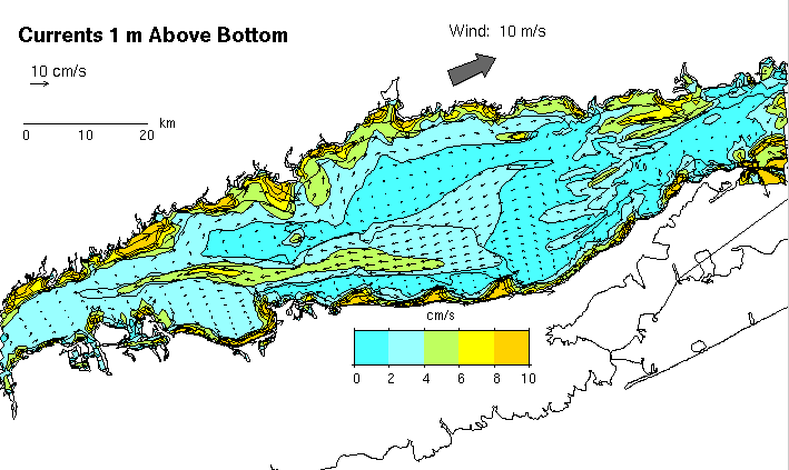 |
| Figure 6. Simulated near-bottom currents (1 m above bottom) during a moderate
west-northwesterly wind event (10 m/s). |
The results of this study provide a general framework of bottom currents in Long Island Sound. In the funnel-shaped eastern part of the Sound, the gradient of tidal-current speeds parallels a westward progression of sedimentary environments (Knebel et al., 1997). Currents here are sufficient to move sediments of fine sand and coarser and to produce coarse lag deposits in areas of erosion or nondeposition as well as winnowed finer sands in areas of bedload transport and sediment sorting. Although the tidal-current regime can explain most general aspects of the distribution of bottom environments, our modeling indicates that the tidal currents are too weak to move sediments along the nearshore margins of the Sound, and sediment transport by waves may be more important. In these shallow regions, the bottom orbital speeds associated with surface waves are strong and are sufficient to resuspend fine-grained sediments (muds) about 1-10% of the time. The frequency of sediment movement drops dramatically with water depth, and waves have essentially no effect in water depths greater than about 20 m. Westerly wind events are shown to locally enhance estuarine and tidal bottom currents along the axial depression of the Sound, providing a possible explanation for the relatively coarse sediments found in the depression. Work is continuing on the development of high-resolution models of bedload and suspended-load transport to further increase our understanding of these processes.
John Evans developed analysis and graphical tools that greatly facilitated this study. Ralph Lewis and Muriel Grim supplied us with bathymetry data that made construction of a high-resolution digital bathymetric grid possible.
Blumberg, A.F. and Mellor, G.L., 1987, A description of a three-dimensional coastal model, in Three-Dimensional Coastal Ocean Models, N. Heaps [ed], Coastal and Estuarine Sciences, v. 4, p. 1-16.
Bokuniewicz, H.J., 1980, Sand transport at the floor of Long Island Sound, Advances in Geophysics, v. 22, p. 107-128.
Bokuniewicz, H.J., and Gordon, R.B., 1980a, Storm and tidal energy in Long Island Sound, Advances in Geophysics, v. 22, p. 41-67.
Bokuniewicz, H.J., and Gordon, R.B., 1980b, Sediment transport and deposition in Long Island Sound, Advances in Geophysics, v. 22, p. 69-106.
Butman, B., 1987, Physical processes causing surficial-sediment movement, in Georges Bank, R.H. Backus [ed.], MIT Press, Chapter 13, p. 147-162.
Csanady, G.T., 1973, Wind-induced barotropic motions in long lakes, Journal of Physical Oceanography, v. 3, 429-438.
Gordon, R.B., 1980, The sedimentary system of Long Island Sound, Advances in Geophysics, v. 22, p. 1-40.
Holthuijsen, L.H., Booij, N., and Herbers, T.H.C., 1989, A prediction model for stationary, short-crested waves in shallow water with ambient currents, Coastal Engineering, v. 13, p. 23-54.
Kenefik, A.M., 1985, Barotropic M2 tides and tidal currents in Long Island Sound: a numerical model, Journal of Coastal Research, v. 1, no. 2, p 117-128.
Knebel, H.J., Rendigs, R.R., Signell, R.P., Poppe, L.T., List, J.H. and Buchholtz ten Brink, M.R., 1997, Seafloor environments in Long Island Sound: implications for contaminant dispersal in a large urbanized estuary (abs): Geological Society of America, Abstracts with Programs, v. 29, no. 6, p. A-90.
Knebel, H.J., Signell, R.P., Rendigs, R.R., Poppe, L.J., and List, J.H., 1998, Seafloor environments in Long Island Sound, manuscript to be submitted to Marine Geology.
Komar, P.D. and Miller, M.C., 1975, Sediment threshold under oscillatory waves, in Proceedings 14th Conference on Coastal Engineering, American Society of Civil Engineers, New York, p. 756-775.
Luettich, R.A, Jr. and Westerink, J.J., 1995, Continental shelf scale convergence studies with a barotropic tidal model, in Quantitative Skill Assessment for Coastal Ocean Models,
D. Lynch and A. Davies [eds.], Coastal and Estuarine Studies Series, v. 48, p. 349-371, American Geophysical Union Press, Washington, D.C.
Schmalz, R.A., 1993, Numerical decomposition of Eulerian residual circulation in Long Island Sound, Proceedings, Third International Conference on Estuarine and Coastal Modeling, ASCE Press, p. 294-308.
Schmalz, R.A., Devine, M.F., and Richardson, P.H., 1994, Residual circulation and thermohaline structure, Long Island Sound Oceanography Project Summary Report, Volume 2, NOAA Technical Report NOS-OES-003, National Oceanic and Atmospheric Administration, Rockville, MD, 199 pages.
Wolfe, D.A., Monahan, R., Stacey, P.E., Farrow, D.R.G., and Robertson, A., 1991,
Environmental quality of Long Island Sound: assessment and management issues, Estuaries,
v.14, p. 224-236.