USGS Home
Contact USGS
Search USGS

A description, comparison to other data, and interpretation of the electromagnetic data from the 1997 Airborne ElectroMagnetic (AEM) survey, Fort Huachuca vicinity, Cochise County, Arizona

by Jeff Wynn

U.S. Geological Survey, Reston, VA 20192

CHAPTER SUMMARY:

GEOTEM is a proprietary, fully digital airborne survey system developed and operated by Geoterrex, LTD, of Ottawa, Canada. CDTs (Conductivity Depth Transforms) are a proprietary product provided at extra cost by Geoterrex. These are calculated conductivity-vs-depth sections derived by mathematical transform of the 120-channel airborne electromagnetic in-phase/quadrature data acquired by the GEOTEM geophysical survey system, using an infinite half-space assumption. We compared the CDT sections first with Vertical Electrical Soundings (VES) carried out in the upper San Pedro Basin and reported in Pool (1998), and second with water-table depths (Tatlow, 1998) and with older well-logs. In general we found good agreement between the CDT information and the VES and well-logs for the first 150 meters below the Earth's surface. We also found good agreement between the CDTs and other sources of San Pedro Basin aquifer information [for instance, Corell et al., 1996). There is excellent correlation between CDTs and water-table depths. When there is a disagreement between the VES soundings and the CDT data, the water-table data support the CDT data. We conclude that the substantive interpretations and maps of the "San Pedro Basin Airborne EM Survey - Preliminary Report" (Wynn and Gettings, 1997) are valid.

BACKGROUND:

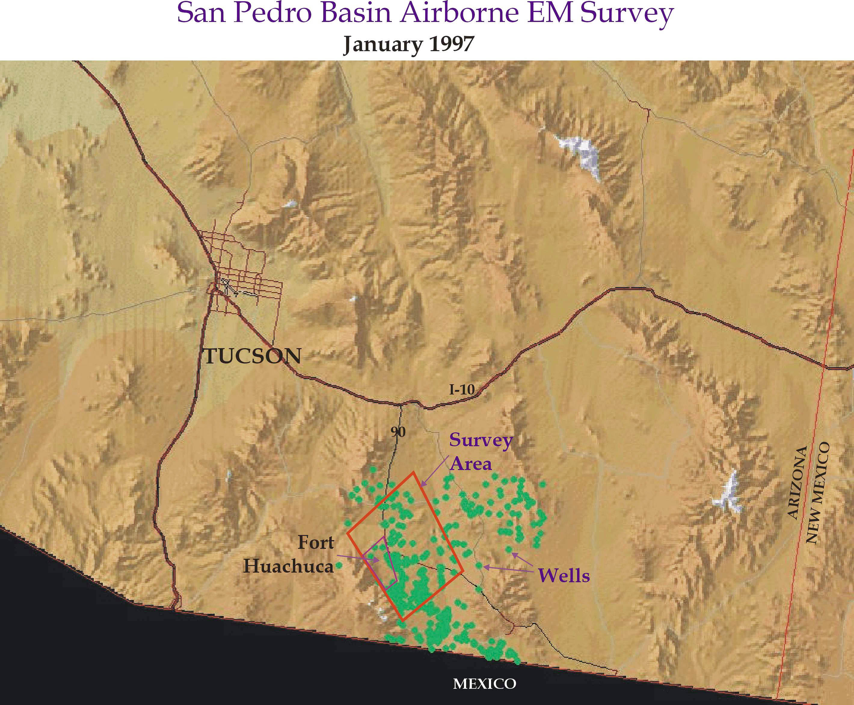
In January 1997 the USGS contracted and supervised a time-domain Airborne ElectroMagnetic (AEM) and magnetic survey over the upper San Pedro River drainage, covering an area roughly 400 square km  in size between Fort Huachuca and the San Pedro River in Cochise County, southeastern Arizona (see index map, figure 1.

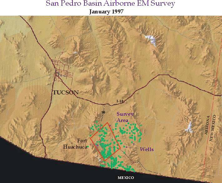
A larger version of figure 1 can be obtained by clicking here).

Using an initial, informal release of raw data from the contractor (Geoterrex Ltd. of Ottawa, Canada), a Preliminary Report was produced for immediate use by the US Army Garrison at Fort Huachuca (Wynn and Gettings, 1997). In an effort to evaluate the final release of data (received by the USGS on 22 March 1998) in more detail, we have examined the airborne multi-channel conductivity map grids, the Conductivity Depth Transforms (CDTs), and the aeromagnetic map grid provided by Geoterrex, Ltd. We have focused our efforts primarily on two areas:

1. Evaluation of the usefulness of the CDTs for mapping the water table between the Huachuca Mountains and the San Pedro River, in the area where significant ground water withdrawal takes place. We did this by comparing the CDTs to the known water-table in key wells, comparing the CDTs to Vertical Electrical Soundings (VES) acquired in the area, and comparing the CDTs to electrical logs of wells in the area.
2. Examination of the aeromagnetic map provided by Geoterrex for its ability to define the shape of the crystalline basement underlying the sediments hosting the San Pedro aquifer. This is the subject of Chapter 1.

Note: in this report conductivities and resistivities are both used, depending on the data under consideration. Well-logs are almost always reported as resistivity vs. depth, whereas most AEM systems report conductivities. Resistivity is simply the inverse of conductivity: rho = 1/conductivity . We have tried throughout this report, whenever possible, to relate the electrical resistivity observed (or calculated in the case of the CDTs) to the lithology and porosity of the underlying rocks and unconsolidated sediments we are mapping.

The Geoterrex GEOTEM System is an airborne GEOphysical Time-domain ElectroMagnetic system comprised of an aircraft (in this case a Brazilian CASA Turboprop) and a set of closely integrated transmitter and receiver coils. The transmitter array consists of six horizontal-loop cables strung from nose to wing to tail to wing to nose on the outside of the aircraft - a total loop area of 232 square meters. This transmitter loop array is driven by a 935-amp (600 amps RMS), half-sine-wave time-domain signal, powered by a generator-transmitter located onboard the aircraft. The received signal (consisting of the primary transmitted signal and the secondary Earth-response signal) is measured by a towed-bird detector with three mutually perpendicular coil axes. The EM bird is towed behind and about 120 meters above the ground during flight. The three receiver-coil axes are sensitive to horizontal conductors (the z-axis), and vertical conductors (x- and y-axes). The x-axis receiver coil couples preferentially to signals arising from vertical conductors whose strike is parallel to the flight direction, while the y-axis responds preferentially to vertical conductors perpendicular to the flight direction. Since the survey was designed to search for water in horizontal and sub-horizontal layering, we focused our analysis on the secondary signal captured by the z-axis coil.

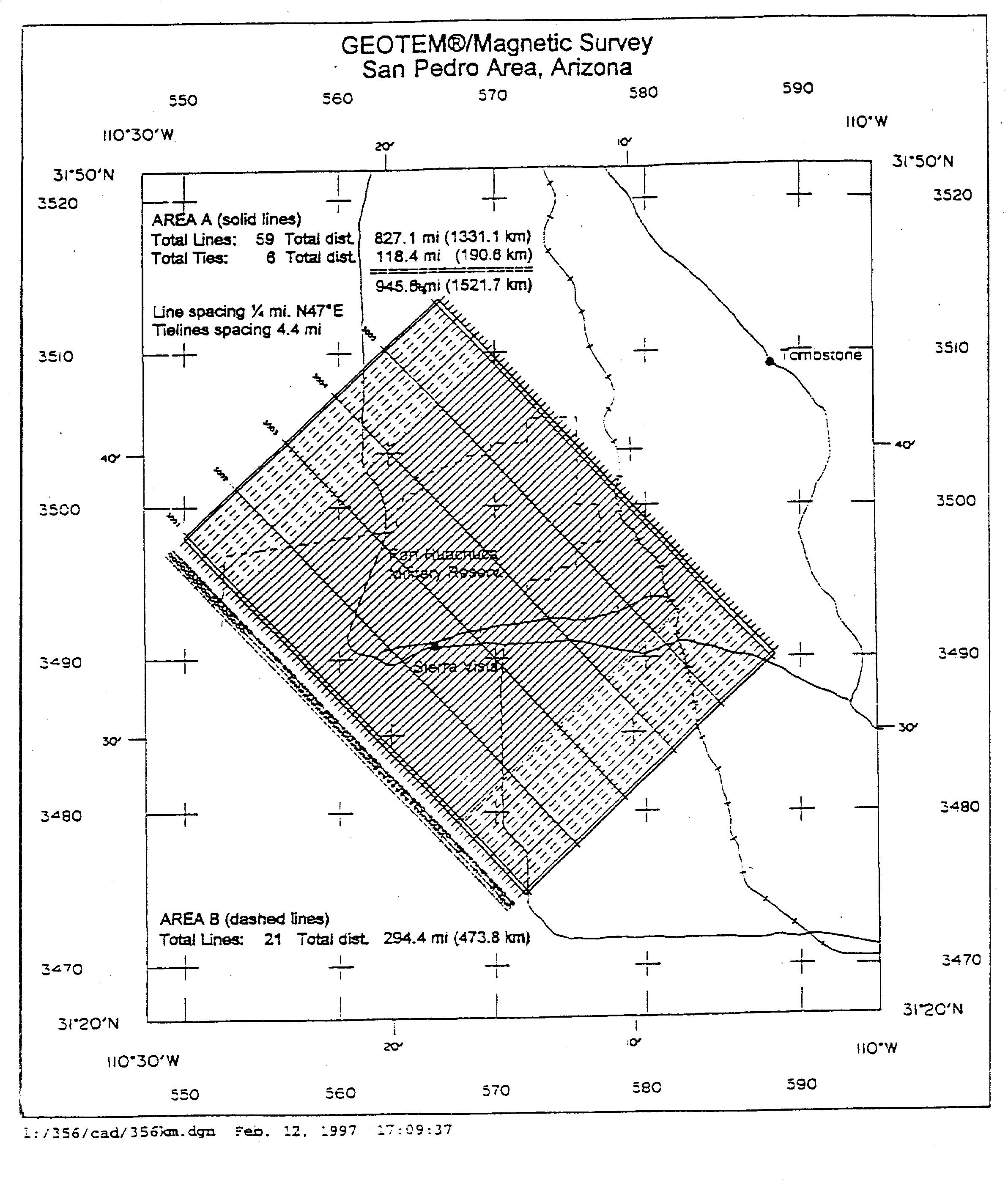
Survey flight lines are described in detail in Chapter 1 on the magnetic survey; the flight lines are shown in figure 2.

A higher-resolution version of Figure 2 can be obtained by clicking here.

For an EM dipole, signal strength falls off as the distance cubed, so it is essential to maintain the transmitter as close to the ground as safety permits. Effective signal penetration-depth also increases with decreasing frequency (which arrives at progressively later times after the initial impulse). Nominal flight (and therefor transmitter) terrain-clearance was thus held at 120 meters (400 ft) except where FAA regulations required 500 ft terrain-clearance over inhabited areas. The EM transmitter operated at the system minimum repetition rate of 30-Hz, giving a pulse width of 4036 /sec. this was done to maximize the penetration of the transmitted signal in an arid, conductive environment. The 3-component multicoil system at this repetition rate is expected to provide conductivity information as well as structural information about the upper 150-200 meters of the subsurface.

Real-time digital processing done on the received signal allows for the efficient removal of the primary signal and effects of aircraft frame flexure and vibration, a process called "compensation". The different time-sampling windows of the resulting residual Earth coupling response thus have a low noise content, which permits effective use of secondary signals from substantial depths. This "gating" also gives an indication of the depth of the source; that is, longer times correlate with deeper sources. The CDT calculation process, based on a forward-modeling signal-correlation algorithm, converts these gated results to discrete conductivities as a function of depth.

THE AIRBORNE CONDUCTIVITY MAPS:

The following maps give resistivities derived from the z-axis receiver coil (the coil preferentially coupled into flat-lying conductors beneath the ground) at different times in the received decay signal. Channel 2 in these representations is the deepest-penetrating channel, while channel 10 is the shallowest represented shown here. Table 1 below shows the mean delay times in microseconds for each channel after the end of the half-sine transmitter pulse.

TABLE 1. Delays in microseconds for each EM channel in the Geoterrex GEOTEM airborne system.

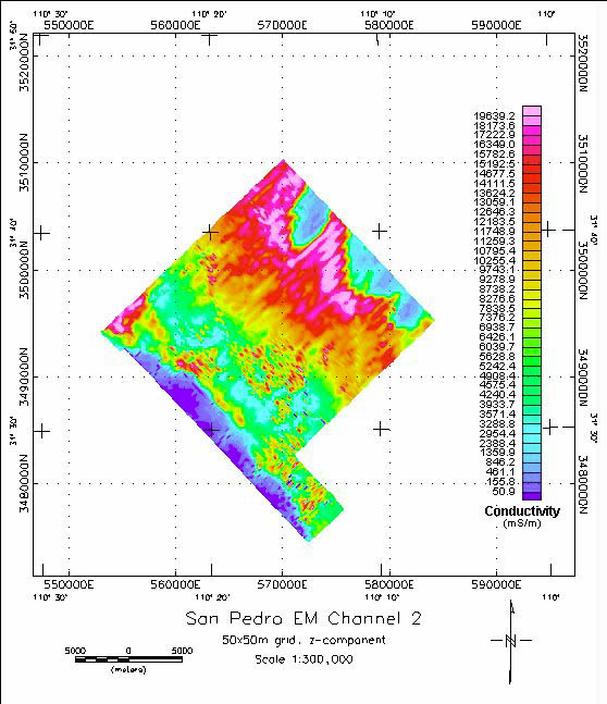Figures 3 shows the conductivities for the z-axis coil for the gated window designated as EM channel 2; this corresponds to the deepest penetration signal. (A higher-resolution version of figure 3 can be seen by clicking here.)

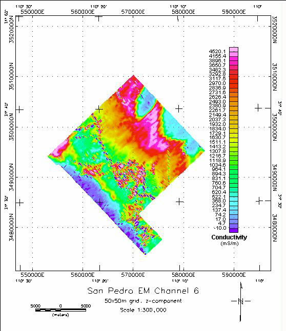
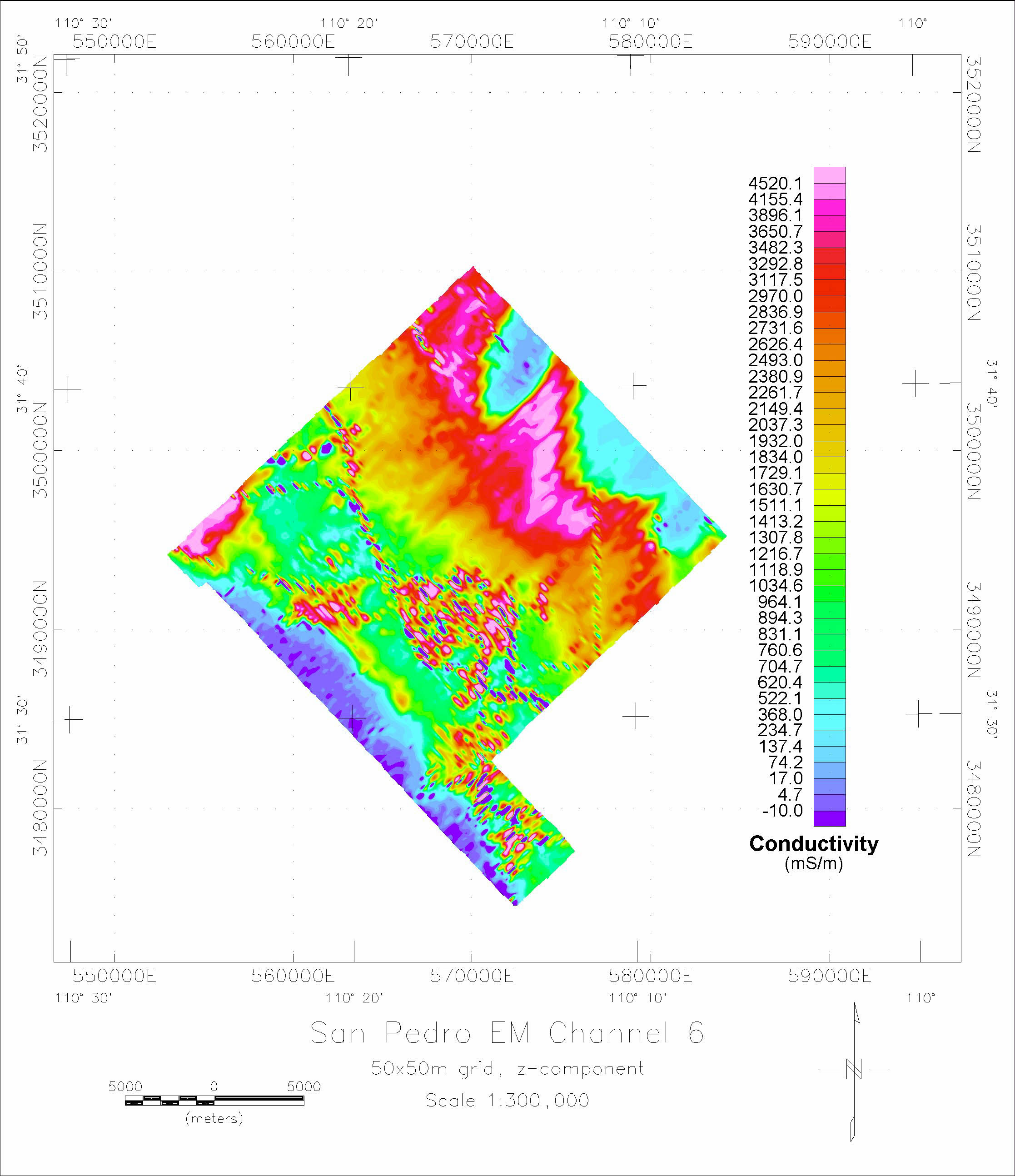
Figures 4 shows the conductivities for the z-axis coil at channel 6, representing an intermediate depth. (A higher-resolution version of figure 4 can be seen by clicking here.)

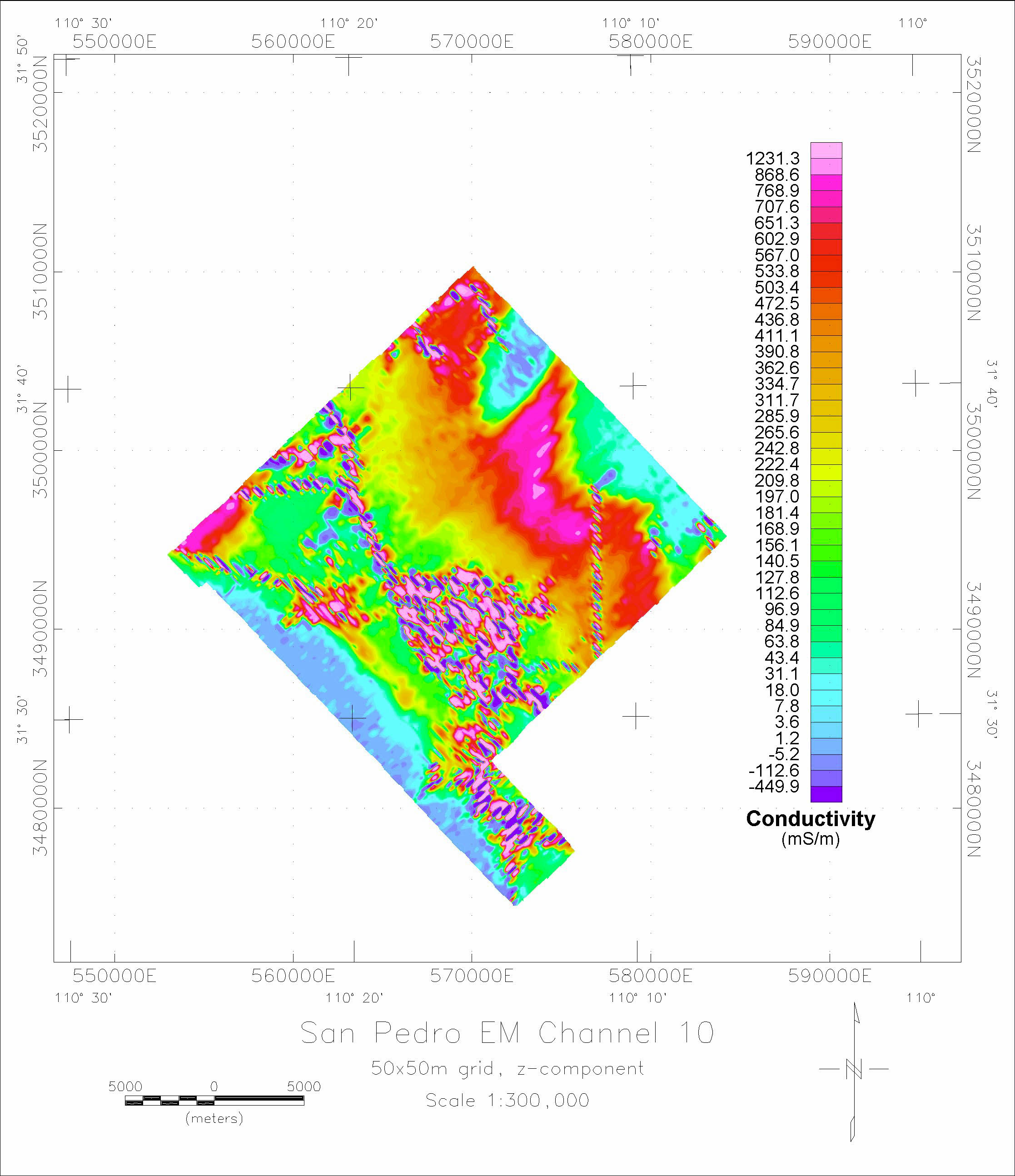
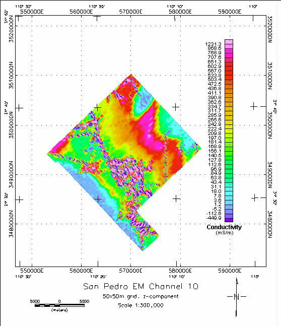Figure 5 shows the conductivities for the z-axis coil for channel10, the shallowest-penetrating channel reported by Geoterrex. Note the strong cultural interference (high-frequency speckling) caused by electrical power lines at Sierra Vista, Fort Huachuca, and along the connecting roads.(A higher-resolution version of figure 5 can be seen by clicking here.)

In effect, these figures can be roughly thought of as depth-slices in the 3-D conductivity of the survey area. Cultural interference is caused by pipelines and grounded powerlines, both of which strongly couple to the high-frequency signals of the AEM transmitter. In the channel 10 z-axis conductivities, Fort Huachuca and Sierra Vista are clearly outlined by this speckling; in the eastern side of the figure a north-south band of speckling apparently represents coupling to the metal structure of an aquaduct. Channel 2 has much less interference from human culture, but residual effects can still be seen even in this channel.

On all three figures, conductivity variations generally reflect water content, which can be used to infer lithologic changes. This association can be attributed principally to changes in porosity, since the conductivity of the ground water is presumed to vary little in the San Pedro Basin. In fact, the source of conductivity variations is not always quite as simple as this; sometimes significant changes in the content of certain types of clays in the aquifer will also affect the conductivities. Some of the differences noted later may be due to changes in clay content as one moves away from the Huachuca Mountains. The southwestern edges of the images show blue (low conductivities), corresponding to the low-porosity crystalline rocks of the Huachuca Mountains. The centers of the figures are dominated by greens, yellows, and reds (conductivities of 5,000 to 20,000 mS/m), generally reflecting the higher water-content of the sediments in the basin. The northeastern parts of the figures are dominated by a systematic variation in conductivities that reflect the presence or absence of exposed rocks of the Tombstone Hills (the blue appearing at the upper right edges). It is clear from these images that the crystalline rocks of the Tombstone Hills extend farther west than shown on the geologic map; in other words, the sediments lap onto shallowly-buried crystalline rocks, covering their western extent with a thin veneer of unconsolidated sediments. Also in these figures, there is a systematic variation in the porosity/water content of the sediments between Sierra Vista and the Tombstone Hills. This variation shows increasing conductivity towards the northwest: this is interpreted as the water table shallowing towards the northwest. This correlates exactly with the known behavior of the water table from the few wells in the area, and verifies that these conductivity maps effectively map the water table in three dimensions. A comparison of the red zones in the channel 2 and the channel 10 data shows that the deeper-penetrating resistivity map (channel 2) also shows abundant water closer to Sierra Vista... in other words the deeper image picks up the deepening aquifer closer to the city as one moves farther southwest.

There are additional subtle offsets in the apparent conductivities in figures 3-5 that are not directly related to the presence of the Tombstone Hills or Huachuca Mountains crystalline rocks. One of these offsets exactly coincides with the mapped location of the Sawmill Canyon Fault (Drewes, 1980). It is reassuring that the AEM data not only agree with the water table (and apparently map it with precision), but also apparently correlate well with other known geologic structures in the area.

It is appropriate here to point out a fundamental difference between the electrical and magnetic datasets. Depth of penetration of AEM (active) systems is a function of distance from the transmitter, whereas depth of penetration for magnetic profiling (passive) systems is a function only of how long the profile is. The geometrical limitations of the GEOTEM system thus permit us to map only the top 150-200 meters of the ground, and with few exceptions cannot see below this, whereas the magnetic data allow us to map the local crystalline basement in some cases as deep as 1 km. The shallower EM data, however, offer us far more information and resolution in the top zones of the aquifer than the magnetic data, which conversely is our exclusive source of information for the deeper zones. Trying to compare the two would be a mistake... like comparing apples and oranges. Instead, the two different datasets compliment each other by providing much more information about different physical properties together than they could if only one or the other were used.

One final observational note should be made here. Recalling that the signal strength of an EM dipole falls off with distance cubed, one effect of the human cultural interference is to overload the dynamic range of the secondary Earth response in the receiver coils. In effect, the weakening-with-depth signal can be overwhelmed in some places by cultural noise. The CDT calculation process includes a data-quality test, and when the noise exceeds the signal, colors are cut off on the bottom of the CDT and the transformation stops calculating conductivity for depths any deeper than this. This is manifested on the CDTs (see Plates 3.1 to 3.4 in Chapter 3) as blackened-out transformations below certain, varying depths. Where the blackened part rises closer to the surface, it means that human cultural interference has overwhelmed the transformation in this area.

COMPARISON DATASETS:

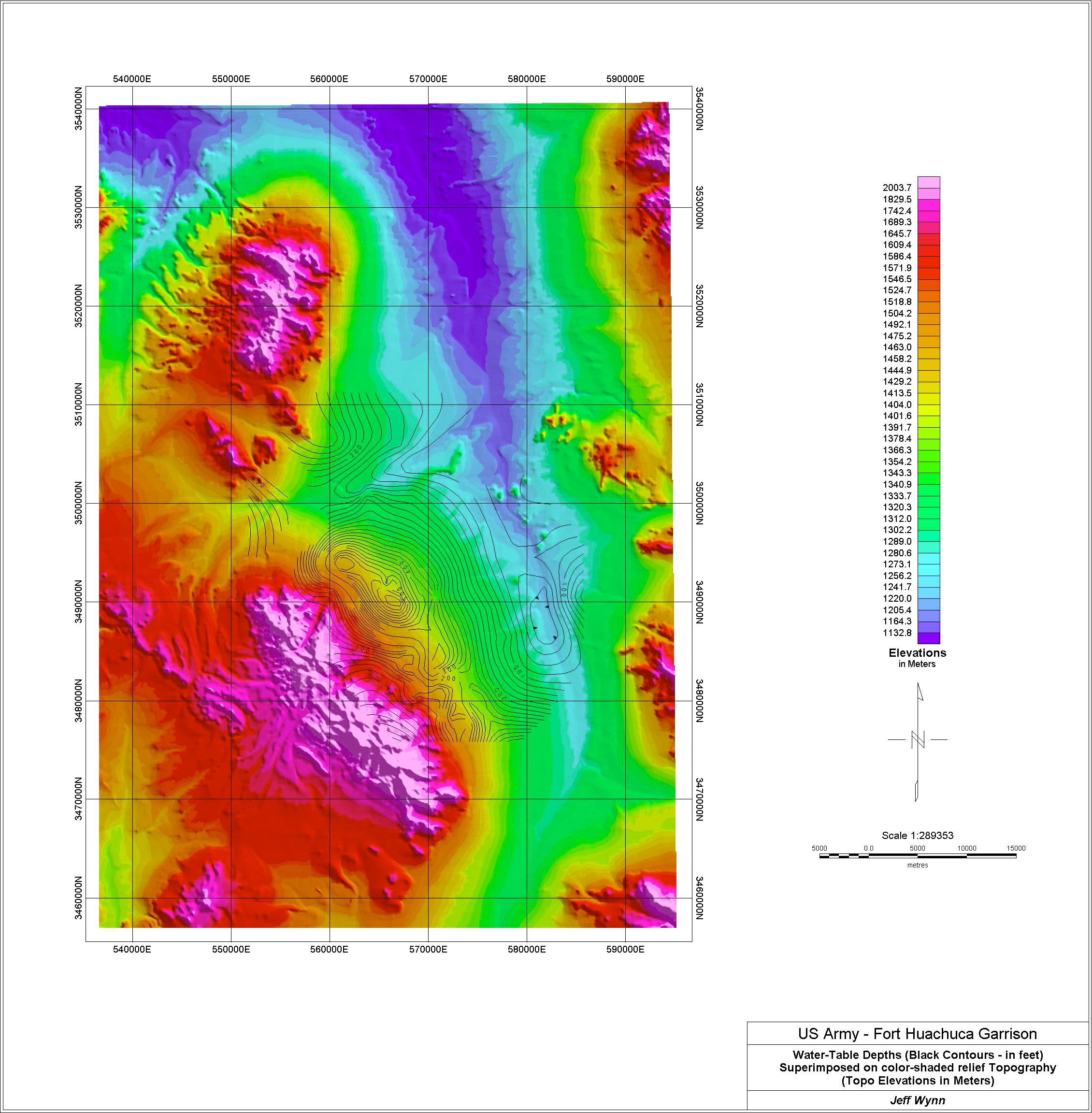
An up-to-date, edited file of water-table information was obtained from Maurice Tatlow of the Arizona Department of Water Resources (Tatlow, 1998; also see Appendix 1). These water table depths are gridded and plotted over the terrain in figure 6.

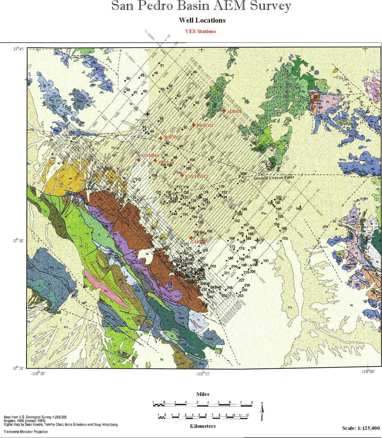
(A higher-resolution version of figure 6 can be seen by clicking here.) Most of these water-table records were narrowed down to the 1996-97 interval so they are most closely correlatable with the ground and airborne electrical data. These wells were geographically registered against the San Pedro Basin geology map (Kneale et al, 1997). Both of these data sources were geographically registered against the Geoterrex flight-lines for the San Pedro airborne EM and magnetic survey. A series of Schlumberger soundings (also known as Vertical Electrical Soundings, or VES) acquired by Pool (US Geological Survey, Water Resources Division Report, 1998) were also registered against the CDT, geology, and well data. This summary registration figure can be seen in Plate 1. Note that figure 6 (above) is a limited-data representation of the water table in the upper San Pedro Basin; figure 7 shows the locations of the VES soundings with respect to the geology and the well-locations

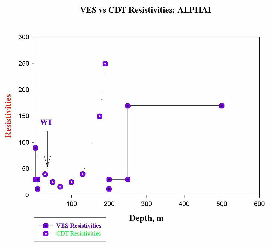
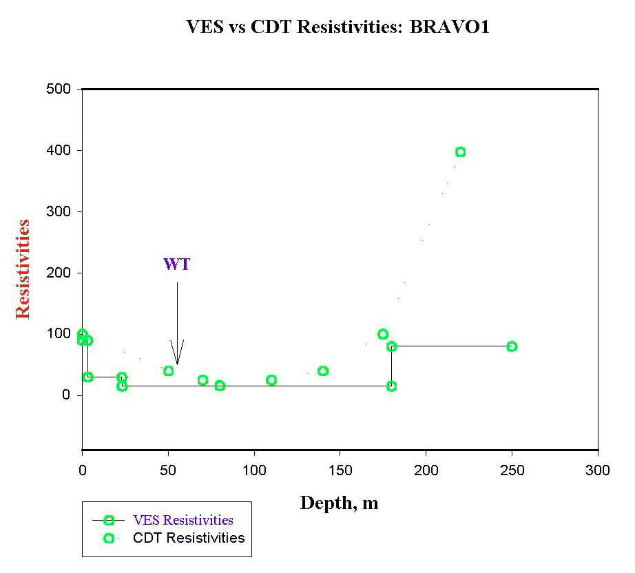
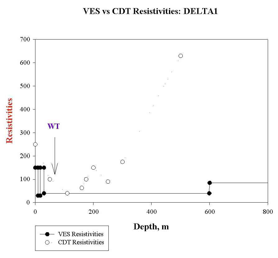
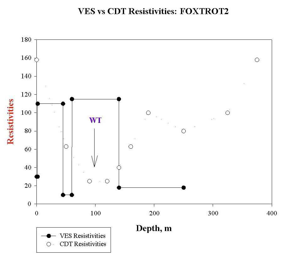
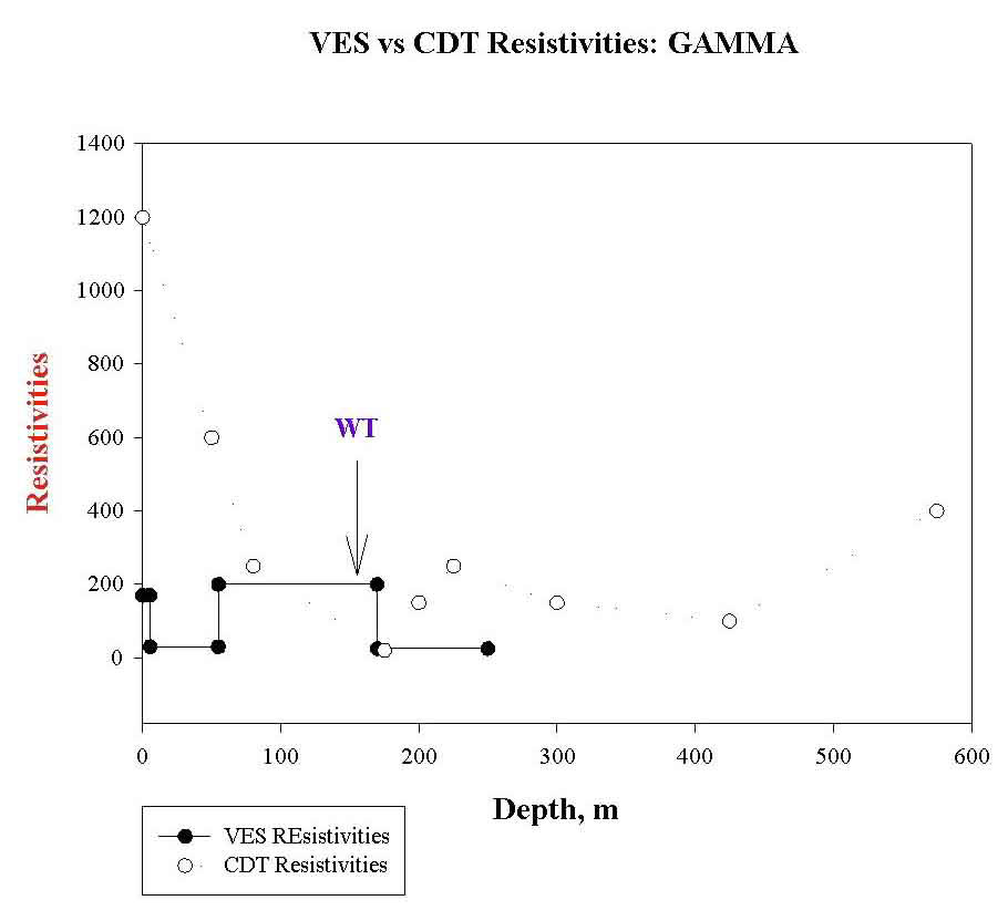
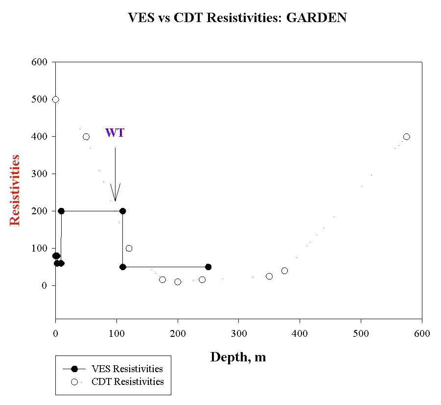
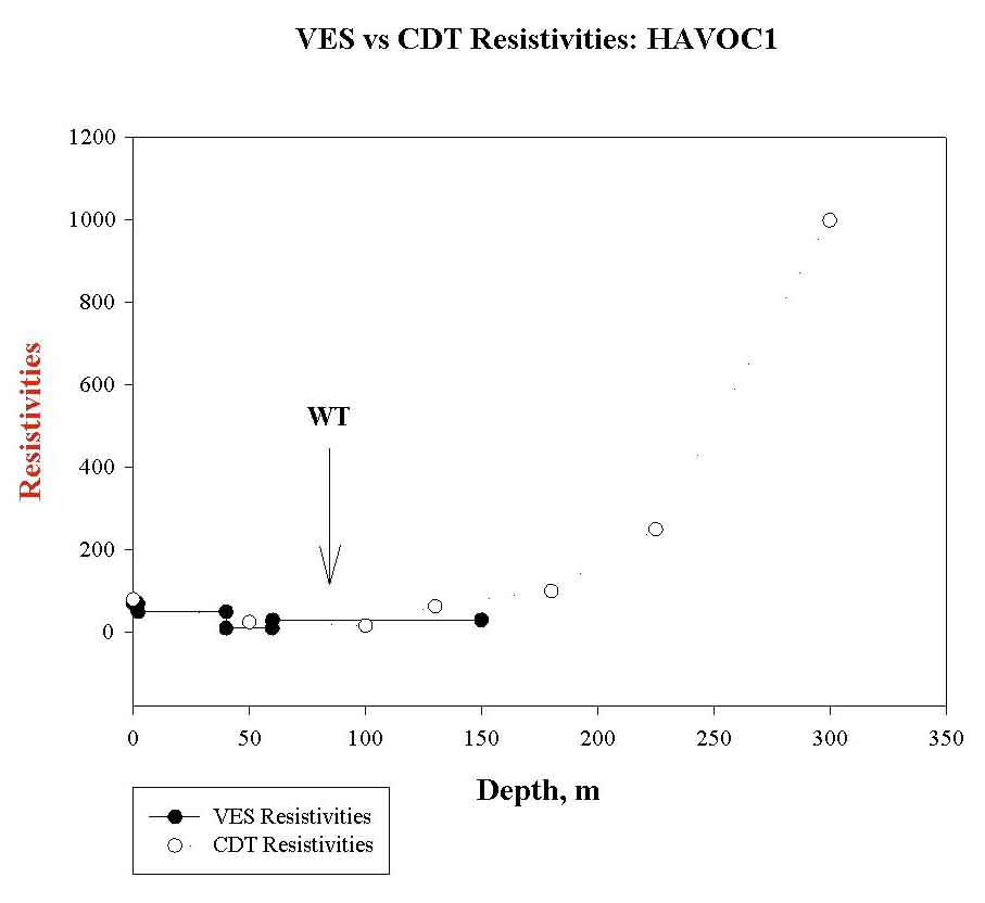
Figures 8-14 show comparisons between vertical CDT profiles, the VES inversions, and the water-table. Brief summaries of these comparisons follow in the table below. Each comparison figure showing CDT, VES inversion, and the water table can be seen by clicking on the appropriate link on the right side of the table. In this table "VES Station" refers to the name given by Pool (1998) to each location (figure 7) where the Schlumber sounding was carried out. "AEM Line" refers to the Geoterrex line number of the closest coincident flight-path, and "AEM Fid" refers to the fiducial, an arbitrary reference point along the line assigned by the Geoterrex data-processing software. The first two numbers of the fiducial refer to the Julian date in which the line was acquired.

Table Comparing VES Inversions and CDTs

GENERAL OBSERVATIONS ON THE VES vs. CDT vs. WATER-TABLE COMPARISONS:

The VES stations were acquired all over the upper San Pedro drainage where the AEM survey was flown, and are therefor a good sampling of the different parts of the San Pedro aquifer. One VES station acquired by Pool (1998) lies outside the bounds of the AEM survey (VES Station "BURN"), and could not be compared with the CDTs. On each figure we have placed an indication of where the water-table lies. These depths are derived from the closest nearby wells. As part of the comparison effort, the depth-to-water-table in the AEM survey area was also plotted using the Tatlow (1998) dataset (Appendix 1; See figure 6). The water table always lies somewhere on the down-going part of the CDT curve, generally between the half-way point and the bottom. It appears to be deeper in the down-going slope in the southwest-central side of the San Pedro basin. Where there is poor correlation between the VES data and the CDT curve, the water table always agrees well with the CDT data. The water-table coincides with the down-going portion of the CDT resistivity curve, almost certainly reflecting the fact that there is an unsaturated but wet vadose zone above the water table that is being picked up by the airborne system. On the basis of this examination, we could use the CDT data (but not the VES data) to draw the water table position to within at least 10 meters of its actual position. This would be highly useful in areas where there are no wells, such as nearby undeveloped basins, or in underdeveloped parts of the San Pedro Basin. One potentiail weakness of using electrical methods of any kind is the fact that there is generally poor contrast between saturated and unsaturated silt and clay.

SUMMARY:

1. The airborne conductivity maps clearly show the presence of the water table and the aquifer in the upper San Pedro Basin. Shallow crystalline basement southwest of the Tombstone Hills is also clearly mapped, along with several left-lateral faults (such as the Sawmill Canyon Fault).
2. The CDTs derived from the 120-channel conductivity data routinely "see" deeper than the VES in site-by-site comparisons. In some cases the CDTs show apparent conductivities down to 600+ meters below the surface, but comparisons with well-logs (Chapter 3 by Bultman and Gettings) show a consistent pattern of higher resistivities below about 150 meters depth, casting doubt on the reliability of the CDTs below 150-200 meters. This considerable depth-penetration (and 150-200 meter depth is excellent by any electrical system standards), is due in part to the fact that the GEOTEM system is very powerful (600 RMS amps, 6 coil-turns, and a huge coil moment-area) and uses sophisticated digital compensation and noise-control. The apparent disparity between the CDT and the well-log resistivities below 150-200 meters is likely due to a systematic error in the way the CDT is calculated for long time-samples. In these comparisons, the VES inversions often didn't penetrate nearly as deep as the CDTs because the AB/2 dipole spacings weren't taken out far enough. The VES work, however, was done before the AEM survey was planned or conducted, and no one knew for certain how deep the CDTs could "see" at that time. Also, because of unavoidable geometric and equipment limitations, the VES equipment (an active-source system) like AEM systems will always provide noisier data at larger AB/2 (receiver dipole) spacings, even if powerlines and fences are not encountered. The noise is simply a consequence of the fact that (A) With larger dipole-spacings, more electrical interference is received, and (B) One can only inject so much current into the VES transmitter dipoles; the bigger the AB/2 distance, the deeper one can theoretically "see", but the smaller the actual detected signal becomes until it converges with the noise threshold. Atmospheric electrical noise ("spherics") increases steadily in the southwestern US as the day progresses, becoming especially strong after about 11 am. If we used large-loop time-domain EM systems on the ground, or a much larger dipole-spacing in the VES soundings, we would also be able to obtain resistivities to these considerable depths. The problem is, it isn't possible to cover 400+ square kilometers at 250-meter spacings in 3-4 days using ground electrical methods.
3. In four of the seven comparison cases, the VES inversions and CDTs correlate well to extremely well. In the three other cases they correlate poorly - or in one case (FOXTROT2) they do not correlate not very well at all. This failure may in part be due to registration errors, but mainly appears to be due to poorly-resolved high-AB/2-spacing data. In other words, the noise threshold is reached early, and there is insufficient information to really resolve the basement features in the VES data (probably because of insufficient current-injection caused by a small VES transmitter). Another way of stating this is that the raw VES data don't support the automatic inversion results for deeper layers in close examination. There may have been some human cultural interference also: the VES raw numbers are suspiciously low in some cases, as if there is a nearby pipeline, cased hole, or grounded fence channeling the input signal.
4. There is a truly remarkable correlation between the CDT conductor tops and the water-table position (see Chapter 3). Where the VES soundings agree poorly with the CDTs the water table depths consistently agree with the top of the CDT conductor. Furthermore, the water-table depths shallow as one progresses northeastward from the Huachuca Mountains to the San Pedro River, and the CDTs show the shallow conductive body (the upper aquifer) getting shallower - also in close agreement with the hydrology in Corell and others (1996). This remarkable correlation has left this author impressed with the usefulness of the CDTs for defining the upper San Pedro aquifer, and probably other aquifers in the southwestern US as well.
5. The accumulated evidence suggests that the Preliminary Report written in April 1997 (Wynn and Gettings, 1997) and submitted to the Army after internal review in late May 1997 is an accurate interpretation for the data available to the US Government at the time. Furthermore, the analysis in this report shows that these conclusions are still valid and hold up to more detailed scrutiny. With the CDT data, however, we can now refine the Corell et al (1996) hydrology even further (see the 3-D imaging in Chapter 3).
6. It seems clear also that the "Deep Conductor" (it should probably be called the "narrow, deep-penetrating vertical conductor on the east") described in the Preliminary Report (Wynn and Gettings, 1997) correlates closely with the mapped edges of the Tombstone Caldera of Moore (1993). In fact, this conductor is a narrow, pervasive, shallow-to-deep feature that goes down at least as far as the CDTs can see along nearly the entire east side of the AEM data.
7. The nature of the "Intermediate Conductor" referred to in the Preliminary Report (Wynn and Gettings, 1997) is still not clear. Further drilling will probably be required to resolve this feature. There are two obvious possibilities: (A) it's caused by a wet, clay-rich body that may be an outflow of the Caldera-collapse event, or (B) it may be a fairly limited-extent, deeper aquifer. The CDTs appear to suggest that it is connected to the shallow conductor over much of its areal extent. An assumption referred to earlier, that the water throughout the San Pedro Basin was of constant conductivity, may not hold in the presence of clays. Clays often increase the conductivity (i.e., lower the resistivity) of water-saturated rocks and sediments.

REFERENCES:

• Corell, Steven W., Corkhill, Frank, Lovvik, Daryl, and Putman, 1996,A groundwater flow model of the Sierra Vista subwatershed of the Upper San Pedro Basin - southeastern Arizona: Arizona Department of Water Resources, Modeling Report No. 10, 107 p.
• Drewes , Harald, 1980, Tectonic Map of Southeast Arizona: USGS MI-Map 1109, 2 plates with text.
• Geoterrex, 1997, Logistics and processing report of the airborne magnetic and GEOTEM electromagnetic multicoil survey over the Fort Huachuca military reservation, cochise County, Arizona: Job No. 356, August 1997, Ottawa, Ontario, Canada, 14 p., 9 Appendices, 2 CD-ROMs with data.
• Kneale, Sean; Bultman, Mark; Chan, Tammy; Grisolano, Anna; and Hirschberg, Doug, 1998, Coronado National Forest Geology, U.S. Geological Survey Administrative Report, CD-ROM.
• Pool, D.R., 1998, in prep., Geophysical investigations near Fort Huachuca, Cochise County, Arizona: US Geological Survey Water-Resources Investigations Report 98-???, 47 p.
• Tatlow, Maurice, 1998, San Pedro Model area well information from GWSI database: written communication, Arizona State Department of Water Resources, 12p., 652 well-measurements. (An edited, adapted version of this table is in Appendix 1)
• Wynn, J.C., and Gettings, M.E., 1997, A Preliminary Interpretation of the 1997 Airborne ElectroMagnetic (EM) Survey over Fort Huachuca, Arizona, and the Upper San Pedro River Basin: US Geological Survey Open File Report OF-97-457, 22 p., 21 figs.