Missouri Department of Natural Resources
Division of Geology and Land Survey
Geological Survey Program
P.O. Box 250
Rolla, MO 65402
Telephone: (573)368-2145
Fax: (573)368-2111
e-mail: nrbakeh@mail.dnr.state.mo.us
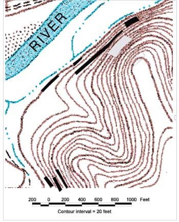
Figure 1. Enlargement of a portion of the Grandin SW 7.5 minute quadrangle showing outcrop polygons for three map units. The four outcrops shown in black, closest to the river are Lower Gasconade Dolomite. The dark gray outcrop in the middle is Upper Gasconade Dolomite and the light gray outcrop at the highest elevation is Roubidoux Formation (the outcrops are normally displayed in easily distinguishable colors). All are of Ordovician age. The outcrop map is the basic map of the field data and is used as the basis for all of the interpreted maps. |
Each map unit is drawn as a separate theme starting from the oldest up. The lowest formation is drawn as a polygon with vertices at only the four corners of the map. Each stratigraphically higher unit is drawn to enclose the areas that lie topographically above its basal contact. In this technique, editing is quick and easy. The themes are merged after editing is complete and before distributing or printing the maps.
Mapping is straightforward in areas where outcrops are abundant, control on contact elevation is good, and the strata are close to horizontal. The contacts can be drawn as bedrock geology polygon themes by following the DRG contours and visually interpolating the elevation between the outcrops, which are color coded for each map unit. Faults are drawn as line themes and the bedrock polygons can be closed on either side of faults or carried across the fault with the appropriate offset depending on the mapper's preference.
In areas where outcrops are widely scattered or sparse and the strata are folded, ArcView is a very useful tool for graphically overlaying different data sets and working them against each other to find the best fit map for all the data. Adding themes for structure and isopach contours was very helpful on one quadrangle where mapping was complicated by a combination of broad folds and map units of variable thickness. With the structural and stratigraphic complications and the complex dendritic drainage pattern, it was difficult to simply "eyeball" the elevation of the contacts correctly between the moderate number of outcrops.
One of the contacts was exposed in several outcrops throughout the quadrangle. By preparing a structure contour map (figure 2) on this horizon and overlaying the structure map on the topography, it was easier to interpret the elevation of the contact. The first step in creating the structure map was to visually scan the outcrops for those where a reliable elevation could be picked and enter those outcrops as a separate point theme with the elevations entered in the attribute table. Each point was then labeled with the elevation. A structure contour map was then drawn as a line theme, using these data points as a base.
In order to draw the bedrock geology polygons, the outcrop theme was turned on with each of the outcrops color coded by formation. The structure contour lines were also color coded to facilitate recognition and make mapping easier. The DRG was placed on top and the white and green colors were made transparent. The bedrock polygons were then drawn with the contact at the correct elevation on the DRG by visually interpolating between the structure contours and the outcrops.
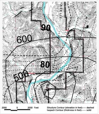
A similar approach was used to draw the contact which overlies a map unit of variable thickness. Because of thickness variations, the contact could not simply be drawn a fixed vertical distance higher throughout the map. In this case, there were enough outcrops where a maximum, minimum, or actual formation thickness could be determined. Those outcrops were entered as a separate point theme and labeled. The isopach maps were drawn as a line theme from these data points (figure 3). Isopach contours were labeled but left black. The contact above this unit of variable thickness could then be drawn by visually interpolating between the structure contours, the isopach contours, and the outcrops (figure 4).
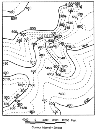
Figure 2. Map of the Grandin SW 7.5 minute quadrangle showing structural control points, and structure contours. |
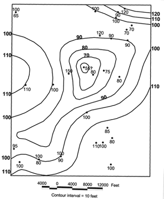
Figure 3. Map of the Grandin SW 7.5 minute quadrangle showing thickness control points and isopach contours of the Upper Gasconade Dolomite. Numbers to the right of the control points are actual thicknesses. Numbers above are maximum thicknesses and numbers below are minimums. |
|
Figure 4. In this clip from near the center of the Grandin SW 7.5 minute quadrangle, the structure map, isopach map, outcrop map, and topographic map are combined to provide control for drawing the formation contacts for the geologic map. The structure contours are color coded with the even 100 foot contours as red and each of the other contours (20, 40, 60, and 80) as other distinct colors that can be easily seen and remembered. This facilitates interpolation between the contours when only 1 or 2 are visible at the scale that the map is being drawn (usually between 1:4000 and 1:8000). The heavy angular line is the boundary of the Ozark National Scenic Riverways. |
Where discrepancies occurred during preparation of the geologic map, the attribute table and field notes were checked first for descriptive information about the outcrops. In some cases, the outcrop observations were identified as being ambiguous or questionable and the outcrop interpretation was changed to fit the structure and isopach maps. If the outcrop data was not ambiguous, the structure and/or the isopach was modified until all of the interpreted maps fit the data. Simultaneously working with these electronic overlays was much easier than working with similar overlays on film or tracing paper.
Experiments are currently underway using AutoCAD Map 3.0 to draw the scaled elements of cross sections. AutoCAD Map has the capability to rotate a DRG. By rotating the DRG until the line of the desired cross section is in a horizontal position, it is possible to place a scaled grid along the line and use the cursor cross hairs to plot the topographic profile and position of geological features. Once the scaled aspects of the drawing are complete, the drawing can be returned to ArcView to fill in detail, text, and color. Other software alternatives are also being reviewed including the use of a USGS DEM in Arc/Info and 3D Analyst ArcView Extension.
The maps drawn in ArcView were the simplest to compile. Individual geologists were responsible for assuring that their maps match along all of the common boundaries. This was easily accomplished in ArcView by adding the shape files from the adjoining quads to each map. Where discrepancies occurred, the geologists involved resolved the problem. In most cases it was a matter of one geologist having control where the other didn't and the map that lacked data was modified to fit with the one with the best control. In a few cases, the discrepancy was a difference in interpretation and occasionally required the geologists to return to the field together and come up with a mutually acceptable interpretation. In either case, the corrected and matched shapefiles were sent to the geologist making the compilation.
The data digitized in GSMAP was more difficult to handle and much less accurate. The data was imported into ArcView as dxf files in the form of polylines, rather than polygons. It was necessary for a technician to close these lines and convert them to polygon themes before the compiling geologist could work with them. The quality of the digitizing varied from excellent to poor and the geologist making the compilation had to frequently refer to the original inked map to determine how to edit the boundary areas to make them match. Another problem was that some of the authors of these early maps are no longer with the Geological Survey Program and could not help with resolving boundary discrepancies. The compiling geologist had to make the best interpretation possible from the existing maps.
Future compilations should be much easier with all of the maps drawn, edited, and matched along the boundaries by the original mapping geologists using ArcView.
The geologists involved in mapping met frequently to develop standards so that all the maps would be as similar as possible. Now that the standards have been established and with the new techniques for the scaled drawings, most of the layouts are being prepared directly by the geologists in ArcView. Composite stratigraphic columns, legends, and templates are being prepared that will allow each geologist to clip those parts that are needed for his or her map and edit them as needed. Drafting support will be minimal.
|
Return to Table of Contents
This site is https://pubs.usgs.gov/openfile/of99-386/baker.html
|