U.S. Geological Survey
National Center, MS 926A
12201 Sunrise Valley Drive
Reston, VA 20192
Telephone: (703) 648-6950
Fax: (703) 648-6953
e-mail: pchirico@usgs.gov
The GIS staff employed a method of scanning, vectorizing, editing, and attributing for digital database creation. Although the process was basically the same for previously published maps, unpublished compiled greenlines, and new mapping compilations, the differences in the original medium required differences in methodology. Previously published maps, which had map separates available, were easily scanned and compiled, whereas greenlines of unpublished data were more difficult to work with.
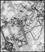
Scans that were made directly from hand drafted compilations of greenline quadrangles contained written text leader lines and other extraneous information that produced complex linework, much of which required deletion (Figure 1a). For new mapping, geologists drafted on mylar that was overlayed on plotted digital basemap files (Figure 1b). These digital basemap files were updated datasets of topographic features and are available in Arc/Info format through the South Carolina Department of Natural Resources, Colombia, South Carolina at http://water.dnr.state.sc.us/gisdata/. In the case of published maps, photographic reproductions of linework were procured for scanning. These black-line positives of scribed linework were ordered from Eastern Region Publications Group of the USGS where some of the scribed map separates still reside. Scans derived from this medium were clean and contained only geologic contact information (Figure 1c).
A |
B |
C |
| Figure 1. Examples of three different geologic data mediums that were digitized. A. Greenline with hand drafted data. B. New hand drafted mylar overlay. C. Black-line positive map separate. | ||
The scanning process utilized an Anatech Eagle 4080 ET large-format scanner, capable of scanning documents up to 40 inches in width. Separates, blackline, and mylar overlays were scanned at different resolutions to provide the best possible file for the vectorization step. Blackline positives are scanned at higher resolutions, between 600 and 800 dots per inch (dpi). Hand drafted greenlines and mylar overlays generally were scanned at 400 dpi. The threshold setting on the scanner regulates the amount of light passing through the medium and therefore affects the clarity of the resulting scan. This threshold setting was altered for each type of media to produce the best possible raster image for vectorization. Blackline positives were scanned using a threshold of approximately 160-180, whereas the hand drafted media needed a higher threshold (190-210) to eliminate some background noise and produce cleaner lines. The raster scans were stored in .tiff or .rlc file format. These raster data formats are accepted by the GTX-OSR (GTX Corporation - Phoenix, Arizona) vectorizing software.
Vectorization of the scanned raster data was a straightforward process and resulting output files of vector linework were saved as Drawing Exchange Format (.dxf) files. Dxf files are easily imported into Arc/Info where the editing process occurs. The editing of vector linework to build topologically correct datasets of geologic polygons and lines was the most important and time comsuming step. Vector linework was projected into the same coordinate system as the digital basemap files (UTM 17, NAD 1927).
Digital basemap files of hydrography and hypsography as well as roads and miscellaneous transportation were downloaded and used as boss layers or backcoverages (drawn on screen in background during the digital editing phase) for the digital compilation. The digital basemap files of hydrography were of particular importance as boss layers for compiling surficial geologic maps because hydrographic and topographic features such as marshes, swamps, mudflats, and islands needed to be copied directly into the new digital geologic coverage. This was done to ensure that geologic and hydrologic features would coincide exactly on future plotted copies and for any subsequent GIS analysis. Hypsography (topographic contour lines) was used in a similar manner. Instead of directly copying lines however, geologic contacts were edited to follow hypsographic lines where required by geologic conditions. For example, geologic contacts describing alluvium and artificial fill were edited to follow the appropriate lines of the topographic backcoverage.
Because the utility of having geologic data in a digital format is the ability to view, query, and analyze the data, a database was developed separately and included a variety of qualitative information that might be useful to data users. A simple database was constructed in Microsoft Access for each of the units depicted on the map. This database was saved as a .dbf file. The .dbf file format was converted into an Arc/Info database file or .info file through the dbaseinfo command. The .info file was then joined to the spatial database with the joinitem command. An explanation of those database items is contained in Appendix 1. An example of the database for surficial geologic map units follows:
| AREA | = 9504.188 |
| PERIMETER | = 376.169 |
| CHAR_GEOL# | = 6 |
| CHAR_GEOL-ID | = 730 |
| MAP_UNIT | = Qwc |
| ID | = 9 |
| UNIT | = Wando Formation |
| FACIES | = clayey sand and clay |
| DEPO_ENV | = backbarrier (estuarine/lagoonal) |
| RELATIVE_AGE | = late Pleistocene |
| MIN_AGE | = 90000.00 |
| MAX_AGE | = 110000.00 |
| ABSOLUTE_AGE | = 90-110 ka |
| LITHOLOGY | = silt |
| MODIFIER_1 | = clayey |
| MODIFIER_2 | = sandy |
| MODIFIER_3 | = very fine-medium |
| MODIFIER_4 | = bioturbated |
| FRESHCOL1 | = pale-yellowish-orange |
| FRESHCOL2 | = medium-light-gray |
| WEATH_COL1 | = grayish-yellow |
| WEATH_COL2 | = dark-yellowish-orange |
| COMPACTION | = moderate |
The final digital databases are stored in an Arc/Info format but are commonly displayed and distributed in an ArcView project. Figure 2 illustrates the combined set of 7.5 minute quadrangles for the northeastern part of Charleston County, South Carolina.
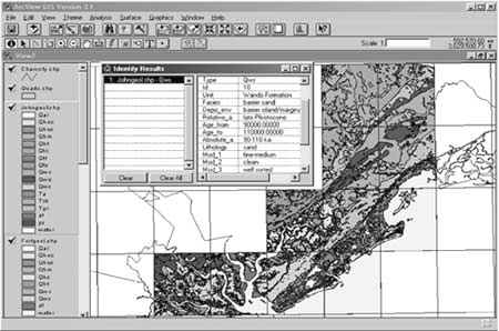
Figure 2. Surficial geologic maps in an ArcView project. |
Data for each corehole includes gamma and electric logs, and lithologic and fossil data. Geologic formations are recognized at different depths throughout the core by analyzing the available data. Depths to each geologic formation are entered into an Access database for each core analyzed. Structure contour maps of any surface can then be prepared through contouring the data for a particular formation. The database is stored in a relational format to prevent duplication of information and to simplify the process of contouring surfaces of selected geologic units. The main data table stores identifier information for each core hole, and examples are shown in Table 1.
| Table 1. Example of the main data table for subsurface geologic information. | ||||||
| USGS_NO | SCWRC_NO | NAME | COUNTY | LATITUDE | LONGITUDE | TOTALDEPTH |
| CHN_635 | 16DD-y3 | Town of Sullivans Island | Charleston | 32.76444 | 79.83278 | 2540.00000 |
| DOR-37 | 23CC-I1 | USGS-Clubhouse Crossroads #1 | Dorchester | 32.88806 | 80.35917 | 2599.00000 |
Ancillary data tables are linked to this identifier table through a common field (USGS_NO) and contain numerical values that show the depth to the top and bottom of the unit and each unit's thickness (Table 2). Several tables are created for each hole, each for a different geologic formation encountered at a different depth in that hole.
| Table 2. Example of ancillary data tables containing information for a particular geologic formation | ||||||
| USGS_NO | DATUM_ELEV | DEPTH_TOP | ELEV_TOP | DEPTH_BASE | ELEV_BASE | THICKNESS |
| BRK-089 | 32.00000 | 328.00000 | -296.00000 | 490.00000 | -458.00000 | 162.00000 |
| BRK-272 | 18.00000 | 541.00000 | -523.00000 | 678.00000 | -660.00000 | 137.00000 |
| CHN-011 | 10.00000 | 749.00000 | -739.00000 | 836.00000 | -826.00000 | 87.00000 |
| CHN-012 | 10.00000 | 752.00000 | -742.00000 | 845.00000 | -835.00000 | 93.00000 |
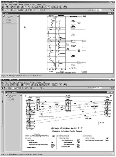
Figure 3. Geophysical logs and cross sections are stored as .dxf files in ArcView database. |
Contour maps were developed for the subsurface geologic units using Arc/Info ver. 7.1.1. Structure contour maps of the top and bottom of each unit as well as an isopach map showing unit thickness were developed. These contour maps were then stored as ArcView shapefiles. The collection of these subsurface layers was stored in ArcView GIS for the traditional two dimensional display structure contour maps. Additional work was then done to include several cross sections to illustrate the regions stratigraphy. Originally these cross sections were created in Micrographix Designer as .dxf files. The .DXF files were then opened in an ArcView View to be displayed (Figure 3).
Future research and development in the use and applications of digital geologic maps will be an important step in the future of digital geologic mapping. Further studies with this dataset include designing maps to include pertinent quantitative data suitable for GIS analysis. Examples for surfical databases include detailed grain size information correlated across geologic units, and blow count or density data for geologic units for some general measure of strength. Geologic map databases must be prepared to address problems of cooperating agencies. In Charleston County, issues ranging from coastal erosion and storm surges, land use planning for growing coastal communities, groundwater resource issues, and further studies related to earthquake hazard and liquefaction potential all require geologic map data to produce viable derivative products.
|
APPENDIX 1. Arc/Info DATABASE DESCRIPTION
Data Format of Database |
|||||
| COLUMN | ITEM NAME | WIDTH | OUTPUT | TYPE | N.DEC |
| 1 | AREA | 4 | 12 | F | 3 |
| 5 | PERIMETER | 4 | 12 | F | 3 |
| 9 | CHAR_GEOL# | 4 | 5 | B | - |
| 13 | CHAR_GEOL-ID | 4 | 5 | B | - |
| 17 | TYPE | 5 | 5 | C | - |
| 22 | ID | 8 | 11 | F | 0 |
| 30 | UNIT | 30 | 30 | C | - |
| 60 | FACIES | 30 | 30 | C | - |
| 90 | DEPO_ENV | 40 | 40 | C | - |
| 130 | RELATIVE_A | 25 | 25 | C | - |
| 155 | MIN_AGE | 8 | 20 | F | 5 |
| 163 | MAX_AGE | 8 | 20 | F | 5 |
| 171 | ABSOLUTE_A | 15 | 15 | C | - |
| 186 | LITHOLOGY | 15 | 15 | C | - |
| 201 | MOD_1 | 20 | 20 | C | - |
| 221 | MOD_2 | 20 | 20 | C | - |
| 241 | MOD_3 | 20 | 20 | C | - |
| 261 | MOD_4 | 20 | 20 | C | - |
| 281 | FRESHCOL1 | 25 | 25 | C | - |
| 306 | FRESHCOL2 | 25 | 25 | C | - |
| 331 | WEA_COL1 | 25 | 25 | C | - |
| 356 | WEA_COL2 | 25 | 25 | C | - |
| 381 | COMPACTION | 15 | 15 | C | - |
ID: Consecutively numbered units.
UNIT: Names of geologic units. Names with upper-case letters are formally defined (for example, Wando Formation). Units with names using lower-case letters are informally defined (for example,Ten Mile Hill beds, artificial fill).
FACIES: General statement of the depositional environment and (or) lithology of a geologic unit. FACIES represents the appearance and characteristics of a sedimentary unit, typically reflecting the conditions of its origin.
DEPOSITIONAL ENVIRONMENT: Describes the environment in which the sediments originally accumulated (for example, estuary,barrier island, marine shelf).
RELATIVE AGE: Age of the geologic units as identified on the standard geologic time scale. Defined in terms relative to other geologic units rather than in terms of years.
MIN_AGE: Numeric field containing the approximate minimum ages of geologic units in thousands of years. This field incorporates the minimum age range from the Absolute Age field but in a numeric form.
MAX_AGE: Numeric field containing the approximate maximum ages of geologic units in thousands of years. This field incorporates the maximum age range from the Absolute Age field but in a numeric form.
ABSOLUTE AGE: Ranges or values for approximate ages of geologic units as determined from fossil ages, amino-acid racemization ages, and (or) radiocarbon ages (ka=thousands of years, Ma=millions of years).
LITHOLOGY: The physical characteristics of rocks or sediments as seen in outcrops, hand samples, or subsurface samples. Described on the basis of characteristics such as color, mineralogic composition, and grain size. Principal sediment types found in the geologic units. Sands consist primarily of quartz grains between 0.0625 mm and 2.0 mm. Silts consist primarily of quartz grains between 0.0039 mm and 0.0625 mm. Limestone/marl deposits consist of true limestone or limy clay (marl). Muck consists of variable percentages of sand, silt, and clay mixed with a high percentage of fine-grained organic material. Descriptions of sediments in the LITHOLOGY and MODIFIER sections are qualitative visual descriptions.
MODIFIER 1, 2, 3, 4: These descriptive terms modify the principal lithologic terms. They are listed in a hierarchical order according to predominant characteristics. Modifiers may refer to size of sand grains (for example, fine-medium), to admixtures of materials of contrasting grain size (for example, silty, sandy, clayey), to special components (for example, fossiliferous, phosphatic), to grain-size sorting (for example, well-sorted, clean), or to stratification type or other fabric characteristics (cross-bedded, bioturbated).
Standard Geologic Grain Size Chart:
- Gravel: larger than 2.0 millimeters
- Sand:
- Very coarse: 1.0 to 2.0 mm
- Coarse: 0.50 to 1.0 mm
- Medium: 0.25 mm to 0.50 mm
- Fine: 0.125 mm to 0.25 mm
- Very fine: 0.0625 mm to 0.125 mm
- Silt: 0.0039 mm to 0.0625 mm
- Clay: smaller than 0.0039 mm
FRESH COLOR 1, 2: Dominant (1) and secondary (2) colors of sediments in fresh exposures and subsurface samples. Color identification was visually determined in the field from the Geological Society of Americas standard color chart.
WEATHERED COLOR 1, 2: Dominant (1) and secondary (2) colors of sediments in weathered exposures. Color identification was visually determined in the field from the Geological Society of Americas standard color chart.
COMPACTION: Qualitative field assessments of sediment compaction stated as "loose", "moderate", or "dense". Younger sediments (Pleistocene and Holocene) tend to be loose or moderately compacted. Older Eocene, Oligocene, and Miocene sediments tend to be dense relative to the younger deposits but still may be penetrated with a knife blade using moderate pressure. (Weems and others 1997).
__________ 1978b, Geological studies of the Charleston, South Carolina area - thickness of overburden map: U.S. Geological Survey Miscellaneous Field Studies Map MF-1021-B, scale 1:250,000
Gohn, G.S., ed., 1983, Studies related to the Charleston, South Carolina earthquake of 1886 - Tectonics and seismicity: U.S. Geological Survey Professional Paper 1313, 375 p.
McCartan, Lucy, Weems, R.E., and Lemon, E.M. Jr., 1980, The Wando Formation (Upper Pleistocene) in the Charleston, South Carolina area, in Sohl, N. F., and Wright, W. B., Changes in stratigraphic nomenclature by the U.S. Geological Survey, 1979: U.S. Geological Survey Bulletin 1502-A, p. A110-A116.
McCartan, Lucy, Weems, R.E., and Lemon, E.M. Jr., 1984, Geology of the area between Charleston and Orangeburg, South Carolina: U.S. Geological Survey Miscellaneous Investigation Series, Map I-1472, scale 1:250,000.
Rankin, D.W. ed, 1977, Studies related to the Charleston, South Carolina, earthquake of 1886 - A preliminary report: U.S. Geological Survey Professional Paper 1028, 204 p.
Weems, R.E., and Lemon, E.M. Jr., 1984a, Geologic map of the Mount Holly Quadrangle, Dorchester and Charleston Counties, South Carolina. U.S. Geological Survey Geologic Quadrangle Map GQ-1579, scale 1:24,000.
Weems, R.E., and Lemon, E.M. Jr., 1984b, Geologic map of the Stallsville Quadrangle, Dorchester and Charleston Counties, South Carolina. U.S. Geological Survey Geologic Quadrangle Map GQ-1581, scale 1:24,000.
Weems, R.E., and Lemon, E.M. Jr., 1987, Geologic map of the Monks Corner Quadrangle, Berkeley County, South Carolina. U.S. Geological Survey Geologic Quadrangle Map GQ-1641, scale 1:24,000.
Weems, R.E., and Lemon, E.M. Jr., 1988, Geologic map of the Ladson Quadrangle, Berkeley, Charleston, and Dorchester Counties, South Carolina. U.S. Geological Survey Geologic Quadrangle Map GQ-1630, scale 1:24,000.
Weems, R.E., and Lemon, E.M. Jr., 1989, Geology of the Bethera, Cordesville, Huger, and Kitteridge Quadrangles, Berkeley County, South Carolina. U.S. Geological Survey Miscellaneous Investigation Map I-1854, scale 1:24,000.
Weems, R.E., and Lemon, E.M. Jr., 1993, Geology of the Cainhoy, Charleston, Fort Moultrie, and North Charleston Quadrangles, Charleston and Berkeley Counties, South Carolina. U.S. Geological Survey Miscellaneous Investigation Map I-1935, scale 1:24,000.
Weems, R.E., and Lemon, E.M. Jr., 1996, Geology of Clubhouse Crossroads and Osborn Quadrangles, Charleston and Dorchester Counties, South Carolina. U.S. Geological Survey Miscellaneous Investigation Map I-2491, scale 1:24,000.
Weems, R.E., Lemon, E.M. Jr., and Chirico, P.G., 1997, Digital Geology and Topography of the Charleston Quadrangle, Charleston and Berkeley Counties, South Carolina. U.S. Geological Survey Open File Series, OF 97-531, scale 1:24,000.
|
Return to Table of Contents
This site is https://pubs.usgs.gov/openfile/of99-386/chirico.html
|