Digital Mapping Techniques '99 -- Workshop Proceedings
U.S. Geological Survey Open-File Report 99-386

Quaternary Landforms in Wisconsin - How Hillshading Can Be Used To Accentuate Topographic Features

Wisconsin Geological and Natural History Survey
3817 Mineral Point Road
Madison, WI 53705-5100
Telephone: (608) 262-2320
Fax: (608) 262-8086
e-mail: dwhankley@facstaff.wisc.edu

The topography of the land surface is a direct result of the type of geologic materials that underlie the surface and the geologic events and processes that acted on them. Therefore, the shape of the land surface can provide important clues to many aspects of the Earth's history.

In contrast to the dominant landforms in the mountainous regions of North America, where topographic relief can exceed 5,000 ft over relatively short distances, the central lowlands of the United States are characterized by relatively low relief topography. Elevations in Wisconsin vary by only 1,500 ft across the entire state, and so Wisconsin landforms tend to be smaller in scale and more difficult to view from a regional or statewide perspective. Glaciated and unglaciated regions dominate Wisconsin's topography, and there are topographic features that are unique to each region.

Throughout the past two million years, continental glaciers repeatedly flowed across much of what is now the northern United States. All but the southwestern quarter of Wisconsin has been covered by ice at different times; most of the glaciated part of the state was glaciated during the Wisconsin Glaciation (Clayton and others, 1991). As the ice sheets advanced and receded, features such as drumlins, eskers, and moraines were formed. Glacial activity was recent enough in many parts of the state to be the dominant influence on the modern landscape.

The effects of stream incision dominate the topography of southwestern Wisconsin, which was never glaciated. Years of drainage have worn down the surface into a highly dendritic network of water channels (Clayton and Attig, 1997).

When evaluating geologic history, a map that effectively displays the way in which topography differs from area to area is usually essential. Topography can be portrayed a number of ways: contour lines, oblique or stereo aerial photography, and shaded relief. Shaded relief maps provide a means of viewing topography that requires little or no interpretation. As an analytical tool, these maps can provide the geologist with a unique regional perspective of topography. The ease with which a shaded relief map can be interpreted also makes it an effective teaching tool. The advent of digital geographic information systems, along with readily available digital elevation data, has made the creation of shaded relief maps fairly straightforward, not the highly interpretive and onerous task it once was. The subtle nature of Wisconsin's topographic variations, especially in the glaciated regions, necessitates the use of a highly detailed elevation model to derive an effective shaded relief map.

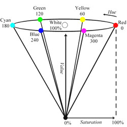
Figure 1. HSV color model (reprinted with permission from ³Specifying Color,² ESRI ArcDoc 7.2.1).

Until recently, statewide digital elevation data were available only in 500-meter and 75-meter raster format; these data were too coarse to show the fine topographic detail that dominates the landscape in the glaciated parts of the state. Complete 30-meter USGS DEM coverage of the state recently became available. The Wisconsin Department of Natural Resources (DNR) compiled the approximately 1,200 30-meter DEMs that make up the state into a seamless grid in Arc/Info.

To derive the hillshading on this map, I used the techniques described by Haugerud and Greenberg (1998). Their methods involve the use of the GRIDCOMPOSITE command with the HSV option in ARCPLOT. This command makes use of the HSV color model, where hue ranges from 0 to 360, saturation from 0 to 100, and value from 0 to 100, as shown in Figure 1. Essentially, GRIDCOMPOSITE combines three grids representing HUE, SATURATION, and VALUE into a composite image. The combination of the analytical power of GRID with the multi-band imaging flexibility of the HSV model results in an effective visual technique.

For this map I wanted the color to be dependent upon elevation. I decided to use a range from green at the lowest elevations to orange at the highest elevations.

I created a HUE grid where the HUE values stretched linearly from green at the lowest elevations to orange at the highest elevation. I had to do the same with the SATURATION grid, only using the SATURATION values that represented my colors. I used the following formulas in GRID:

<HUE_GRID> = [H_LOW] - [H_LOW - H_HIGH] * ((<DEM> - DEM_MIN) / (DEM_MAX - DE_MIN))

and

<SATURATION_GRID> = [S_LOW] - [S_LOW - S_HIGH] * ((<DEM> - DEM_MIN) / (DEM_MAX - DEM_MIN))

where:

[H_LOW] is the Hue component of the HSV color representing the lowest elevations;

[H_HIGH] is the Hue component of the HSV color representing the highest elevations;

[S_LOW] is the Saturation component of the HSV color representing the lowest elevations;

[S_HIGH] is the Saturation component of the HSV color representing the highest elevations;

DEM_MIN is the minimum elevation; and

DEM_MAX is the maximum elevation.

In the HSV color model, color is mainly dependent upon the H and the S values (just as in CMYK, color is mainly a function of C, M, and Y). In this technique, the VALUE grid controls the hillshade effect. Consider that for any pixel of color specified by HUE and SATURATION, the VALUE component sets the amount of black. For instance, a HUE of 120 and a SATURATION of 50 will specify a medium light green. If the VALUE is 0, the resultant HSV color will be black. Similarly, if the VALUE is 100, the resultant color will be the medium light green with no black as a part of the color. This is the effect of shading - shaded areas are blacker than illuminated areas.

Haugerud and Greenberg (1998) note that the contrast of most images produced by the HILLSHADE command in Arc/Info is not suitable for use in this process. They suggest modifying the standard hillshade via the following technique:

&describe <hill_shade_grid>
xxg1 = (<hill_shade_grid> - [Value GRD$MEAN]) * 15 / [value GRD$STDV] + 95)

Because GRIDS in Arc/Info are always rectangular, I had to manipulate the NODATA cells so that they would not print black. I found that the easiest way to do this was to convert the NODATA areas of the HUE, SATURATION, and VALUE grids into a white color. In HSV, white is any H value, S = 0, and V = 100. Using conditional statements in GRID, I converted the values of the HUE, SATURATION, and VALUE grids to their white equivalent wherever the original DEM was NODATA.

The final step in this process was to convert the three grids into a geo-referenced TIF image. The geo-referenced TIF draws faster than the three grid composite and can be displayed in ArcView. To create the image from my HUE, SATURATION, and VALUE grids, I first created RED, BLUE, and GREEN grids using the HSV2RED, HSV2BLUE, and HSV2GREEN commands. I then combined the three grids into a stack using the MAKESTACK command using the LIST option. Finally, I used the GRIDIMAGE command to convert the STACK into a TIF image.

I have attached the AML I used for this process in the appendix.

REFERENCES

Haugerud, Ralph, and Greenberg, H.M., 1998, Recipes for Digital Cartography: Cooking with DEMs, in Soller, D.R., ed., Digital Mapping Techniques '98--Workshop Proceedings: U.S. Geological Survey Open File Report 98-487, p. 119-126, https://pubs.usgs.gov/openfile/of98-487/haug2.html.

APPENDIX

&return &error Bailing out of HSV.aml

Return to Table of Contents This site is https://pubs.usgs.gov/openfile/of99-386/hankley.html Maintained by the Eastern Publications Group Web Team Last revised 11-2-99