Surficial Seafloor Geology of a Shelf-edge Area
off West Florida
by
Kathryn M. Scanlon
Introduction
The U.S. Geological Survey (USGS), in cooperation
with the National Oceanographic and Atmospheric Administration’s (NOAA) National Marine Fisheries Service (NMFS), and Florida State University (FSU), collected the data presented here as part of a larger
study of seafloor habitats on the shelf edge of the northeastern Gulf of Mexico. It is a
pilot study, carried out to demonstrate the utility of geologic mapping to fisheries
management issues. This report contains sidescan-sonar mosaics, seismic-reflection
profiles, texture and calcium carbonate content of sediment samples and interpretative
maps of the seafloor morphology, sediments, and benthic habitats of the study area.
The study area is an approximately 150-km2 area
along the shelf edge in the northeastern Gulf of Mexico. The site is on the eastern side
of the DeSoto Canyon and 75 km due south of Cape San Blas on the Florida panhandle. Water
depth ranges from about 50 meters (m) to 120 m. It was chosen because reports from
fishermen suggested that high-relief rocky outcrops, which are preferred by gag grouper as
spawning aggregation sites, would be abundant. The geologic maps help the fisheries
biologists select station locations for ongoing monitoring studies and provide a basis for
siting of future reserves.
Methods
Three types of data were collected for the mapping effort: sidescan-sonar imagery,
bathymetric and subbottom profiles and sediment samples. In 1997, during a cruise of the
NOAA R/V Chapman, continuous coverage sidescan-sonar images of the entire study
area were collected and subsequently mosaicked. 3.5 kHz echo-sounder profiles were
collected along all the sidescan-sonar tracklines and Geopulse high-resolution
seismic–reflection profiles were collected along some of the ship's tracklines. During several cruises in 1997 and
1998, sediment grab samples were collected from the study area
and analyzed for texture and calcium carbonate content.
Sidescan-Sonar Data Collection and Processing
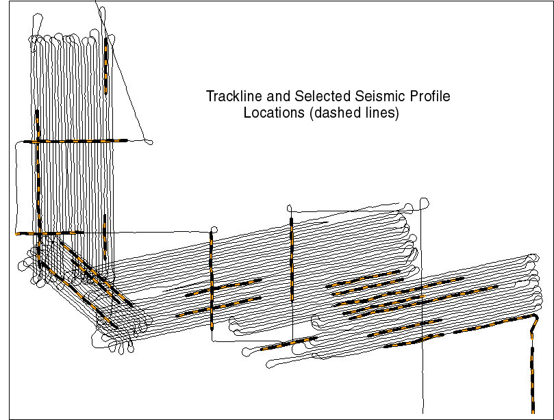
About 1200 line-kilometers of sidescan-sonar data were collected along tracklines
spaced about 167 meters apart, giving sufficient overlap of the adjacent 200-meter swaths
(100 m to each side of nadir) for digital mosaicking. The sidescan-sonar towfish was towed
from a crane off the starboard side of the ship at a speed of approximately 3.5 to 4.0
kts. The sidescan-sonar data and depth along the trackline were recorded digitally.
Ship navigation for the sidescan-sonar tracklines was by Global Positioning System
(GPS). It is estimated that the ship’s position was known to within 10 to 20 m. The
offset between the ship's position and the position of the sidescan-sonar towfish was
estimated based on the length of cable out and by correlation of distinctive seafloor
features in overlapping swaths. The digital navigation data are included in the navigation
files.
Sidescan-sonar data were acquired through use of an EdgeTech
DF1000 sidescan-sonar system, and Isis topside acquisition system, at a rate of 7.5
pings/second, yielding a 200-m (100 m to each side) swath width. The data were decimated
to a 0.4-m pixel size using a median filtering routine developed by Malinverno and others
(1990). They were then processed using procedures developed by Danforth and others (1991)
and Danforth (1997) which include corrections to the slant range (to remove the water
column artifact and convert slant-range distance to true ground distance), destriping (to
correct minor striping noise or dropouts), and beam angle (to correct variations in beam
intensity). Further processing using the routines developed by Chavez (1986), as modified
by Paskevich (1992) for application to high-frequency sidescan-sonar imagery, was
performed to remove additional noise and to orient each sidescan-sonar line in geographic
space. Digital mosaicking was accomplished using the PCI Remote Sensing software package
as described by Paskevich (1996). This dataset was mapped at a resolution of 1m/pixel in a
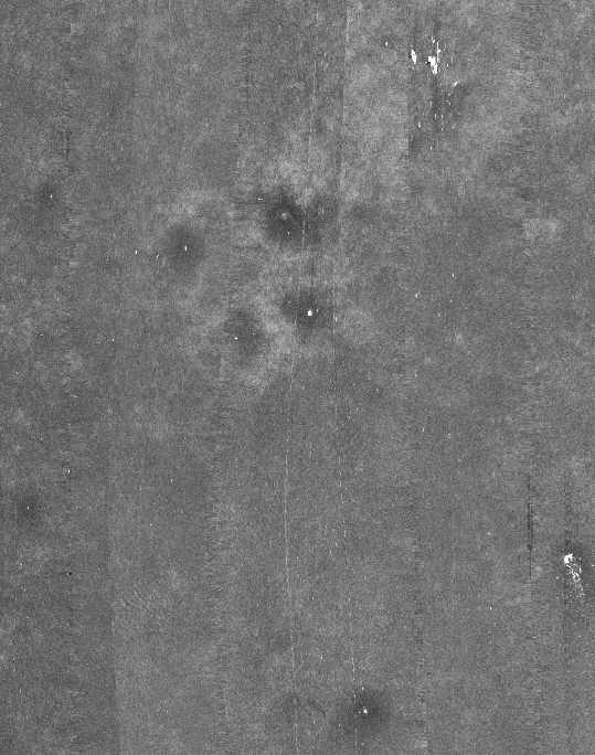
UTM zone 16 projection with the WGS84 ellipsoid. Darker tones on the sidescan-sonar images
represent areas of relatively low acoustic-backscatter intensity and lighter tones, areas
of high backscatter.
Seismic-reflection profile and 3.5.kHz echo-sounder data
Over 500 line-kilometers of high-resolution seismic-reflection
profile data were collected using a Geopulse boomer towed at 1.2 m below the sea
surface off the port side of the ship. The 300-joule boomer was set to a 1/2-second firing
rate and was filtered at 300 Hz to 3 kHz. Penetrations of up to 0.07 seconds of 2-way
travel-time (equivalent to several 10’s of meters of sediment thickness, depending on
the properties of the sediment) were achieved in some areas. About 1200 line-kilometers of
echo-sounder data were also collected using a 3.5 kHz side-mounted system. Both sets of
profile data were collected simultaneously with the sidescan-sonar data and were recorded
on a flatbed paper recorder.
Sediment data
In 1997, four surficial sediment grab samples were collected by C. Koenig during a
cruise of the NOAA R/V Chapman. In 1998, an additional 51 sediment grab samples
were collected by C. Gledhill during a cruise of the R/V Chapman and 3 by G.
Fitzhugh during a cruise of the R/V Carretta. All samples were collected using a
van Veen grab sampler. All samples (except those that were made up of chunks of coral or
coral rubble) were analyzed for particle size and carbonate content in the sedimentology
laboratory of the U.S.G.S. at Woods Hole, Massachusetts. Texture terminology used in this
report is according to Folk (1974). The percent of calcium carbonate material was
determined by weight loss of 15 grams of bulk material after digestion with 10 percent
hydrochloric acid. Details of the laboratory techniques can be found in Appendix I: Sediment Texture Analysis Techniques. The data are
presented in Appendix II: Table of Sediment Analyses.
Interpretation
Based on the sidescan-sonar mosaics, the subbottom seismic-reflection and echo-sounder
profiles and analyses of sediment samples, we have mapped four
distinct bottom types in the study area. Two of the bottom types are defined by the
texture of the sediment cover (coarse sand or silty sand) and cover most of the study
area. The other two bottom types (rocky outcrop and hardbottom) lack or have little
sediment cover. We also mapped three additional seafloor features of significance as
benthic habitats: sand waves, shallow pits and man-made objects. Throughout this document
we use the terminology of Folk (1974) to describe sediment textures.
Medium to Coarse Sand
Most (about 80%) of the sedimented parts of the study area are covered by gravelly or
slightly gravelly medium to coarse sand. The distribution of grain sizes ranges from 3 phi
to –2 phi (phi classes containing greater than 1% of the sample) and peaks at 1 to 2
phi. Typically, the predominant grain composition is quartz and the samples contain less
than 50% CaCO3. These sediments are similar to relict shallow-water Pleistocene deposits,
found in bands throughout the outer shelf environment of the Gulf of Mexico (Poag, 1981;
Gould and Stewart, 1953). Preliminary studies of foraminifera in our sediment samples
confirm that they were originally deposited during the Pleistocene in a shallow-water
environment (W. Poag, pers. commun.). The presence of sand waves (described below)
suggests that parts of this relict sand body are mobile.
Silty sand
The upper slope (depth greater than about 90 m) is covered with finer-grained sediment
(silty sand) and constitutes about 20% of the sedimented parts of the study area. Grain
size distributions of these samples typically range from 6 phi to 1 phi (phi classes
containing greater than 1% of the sample) with a peak at 3 to 4 phi. Silt plus clay
constitutes 5% to 35% of these samples. Most contain minor amounts of gravel. Visual
inspection determined that these samples are generally more cohesive than the medium to
coarse sands.
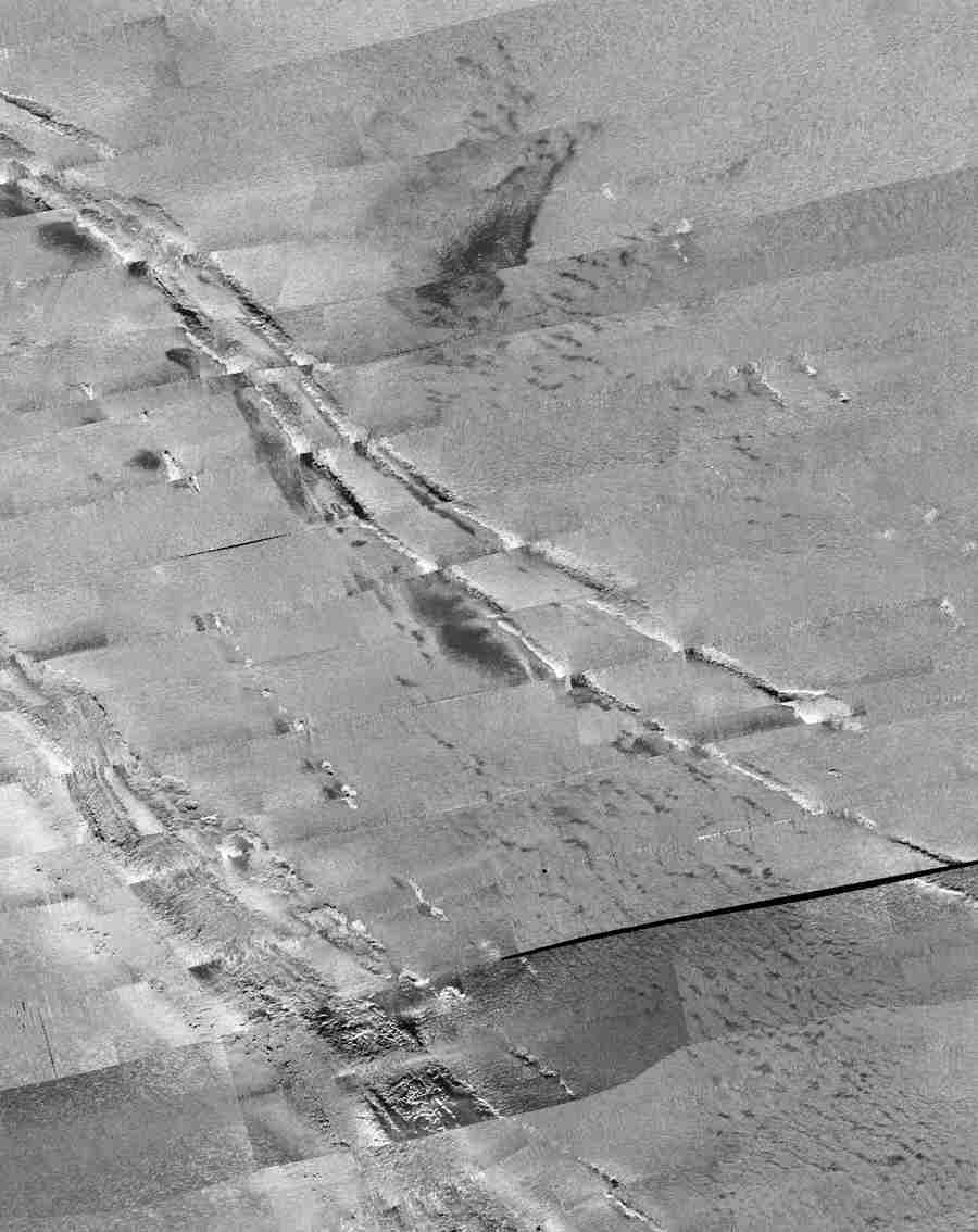
High-relief outcrops
Two pronounced sub-parallel, rocky ledges with up to 15 m of relief were discovered in
water depths of about 60 to 75 m. The ridges trend NW, roughly parallel to the present
coastline of western Florida. The outcrops range from about 40 meters wide to about 200
meters wide and are continuously exposed at the seafloor for up to 5 km in length. Some
can be detected in the subsurface in the seismic-reflection or 3.5.kHz data and followed
for several more kilometers. A single line of sidescan-sonar and seismic-reflection data
collected south of the study area detected additional outcrops with similar character and
orientation as much as 6 km south of the study area. These high-relief rocky outcrops
account for less than 1% of the surveyed area.
Hard bottom
Near the high-relief rocky ledges we found low-relief hard bottom. Because our data
cannot resolve sediment thickness of less than about 1 m, areas mapped as hardbottom may
be overlain by a veneer of unconsolidated sediment. Indeed, we were able to obtain
sediment grab samples at several "hardbottom" sites. This type of bottom is
found over about 7% of the study area.
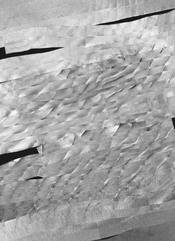
Sand waves
Sand waves occur in patches throughout the medium- to coarse-sand-covered parts of the
study area. Most of the sand waves are in water depths between 60 m and 90 m, but they
extend to over 100 m on the steep south-facing slope of the central part of the study
area. The sand waves vary in dimensions, but generally have a period of 50 to 200 m and an
amplitude of 1 to 4 m (Scanlon and others, 1998) The orientation of the crests of these
bedforms is predominantly NE-SW, but in places is N-S or NW-SE, suggesting complex
currents and, consequently, a complex sediment transport pattern.
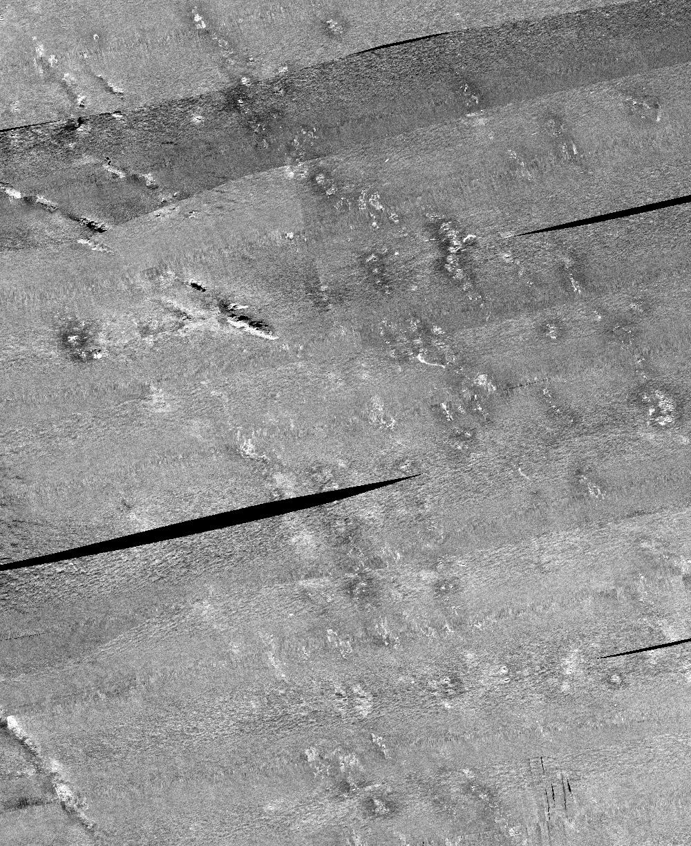
Shallow pits
In the deepest parts of the study area (deeper than 110 m) the sea floor is marked by
numerous shallow (less than 1 m below the surrounding sea floor) pits. Each pit is about 2
m in diameter. They only occur in the silty sand, never in the medium to coarse sand,
which is less cohesive and would collapse more quickly. We presume them to be burrows dug
by tilefish (Branchiostegidae) or yellow-edge grouper (Epinephelus flavolimbatus).
Man-made (?) objects
We also found evidence of numerous hard objects on the seafloor. These objects are
mostly small (1 to 10 m) roughly equant and give a characteristic strong backscatter
signal. Some are surrounded by a circle up to a few 10’s of meters in diameter of low
backscatter in the sidescan-sonar data. The low backscatter halo may be caused by
disturbance of the sediment by fish, which tend to congregate around any hard object on
the sea floor. Some of the larger objects (5 to 20 m, and one about 60 m in length) appear
to be ship wrecks and associated debris. Other objects may have been placed to serve as
"artificial reefs" by fishermen. The resolution of the sidescan-sonar images is
too low to identify these objects – direct observations from a submersible or by
camera are needed to confirm this interpretation.
Conclusions
Before this study, only the gross morphology (as depicted in 1:250,000 scale NOS
charts) of the West Florida shelf edge was known. This pilot study of a small part of the
shelf edge has revealed details that are important to the management of fishery resources.
Perhaps the most important discovery is the existence of the rocky ridges in the
eastern part of the study area. Although they are 15 m high in places and several
kilometers long, they were not previously known. This is the type of habitat that many
deep-water reef fishes, such as groupers and snappers, use for spawning and/or feeding
(Coleman and others, 1996; Koenig and Coleman, 1998). Fisheries biologists need to know
whether their monitoring stations are near fish-attracting outcrops or in a large field of
mobile sand waves. Similarly, the occurrence of numerous unidentified manmade (?) objects
in parts of the study area could be attracting reef fish to areas that would otherwise
lack those species. The discovery of presumed fish burrows in the deeper parts of the
study area confirms the presence of burrowing fish in the area and suggests that they may
be more numerous than previously thought. These pits also are a good indicator of the
composition of the sediment, since they do not occur in the coarser sands.
Fisheries managers in the Gulf of Mexico are increasingly interested in using no-take
reserves to help bolster the populations of over-fished species (Koenig and others, in
press). When creating a reserve, it is imperative to know that the boundaries will
encompass the types of habitat needed by the species that the reserve is intended to
protect. It is clear from this study that existing maps in the shelf-edge areas of the
eastern Gulf of Mexico are inadequate for this purpose and more detailed mapping of
sea-floor habitats, such as this study, are necessary for management decisions.
Acknowledgements:
Many people were instrumental in the collection, processing and publication of these
data. We would particularly like to thank the Captain and crew of the NOAA ships R/V
Chapman and R/V Carretta. J. Denny (USGS) and V. Cross (USGS) processed and
mosaicked the sidescan-sonar data and K. Parolski (USGS) orchestrated the shipboard data
acquisition (sidescan-sonar and boomer). S. Harrison (USGS) and C. Harper (NOAA, Stennis
Space Center), provided shipboard support. D. Blackwood (USGS) and J. Zwinakis (USGS)
contributed photography and drafting skills. A. Robinson (USGS) and B. Taylor (USGS)
did the sediment analyses and J. Reynolds (USGS) assisted with analyses and data entry.
References
Chavez, P.S., Jr., 1986, Processing techniques for digital sonar images from GLORIA:
Photogrammetric Engineering and Remote Sensing, v. 52, no. 8, p.1133-1145.
Coleman, F.C., C.C. Koenig, and Collins, L.A., 1996, Reproductive styles of
shallow-water grouper (Pisces: Serranidae) in the eastern Gulf of Mexico and the
consequences of fishing spawning aggregations. Environmental Biology of Fishes 47:129-141.
Danforth, W.W., O'Brien, T.F., and Schwab, W.C., 1991, Near real-time mosaics from
high-resolution sidescan-sonar - an image processing technique to produce hard-copy
mosaics 'on site' proved successful during USGS survey, Sea Technology, V.32, no.1,
pp54-59.
Danforth, W.W, 1997, Xsonar/ShowImage: A complete system for rapid sidescan-sonar
processing and display, USGS Open-File Report 97-686, pp. 77.
Folk, R.L., 1974, Petrology of sedimentary rocks. Hemphill Publishing Co., Austin, TX,
182 p.
Gould, H.R., and Stewart, R.H., 1953, Continental terrace sediments in the northeastern
Gulf of Mexico, Finding Ancient Shorelines, SEPM, p. 2-18.
Koenig, C. C. and Coleman, F.C., 1998, Absolute abundance and survival of juvenile gags
in seagrass beds of the northeastern Gulf of Mexico. Trans. Amer. Fish. Soc. 127: 44
– 55.
Koenig, C.C., Coleman, F.C., Fitzhugh, G.R., Gledhill, C.T., Scanlon, K.M., Grace, M.,
and Grimes, C.B., in press. Networks of marine reserves for the conservation of warm
temperate reef systems of the southeastern United States, Bulletin of Marine Science.
Malinverno, A., Edwards, M., and Ryan, W.B.F., 1990, Processing of SeaMARC swath sonar
data: IEEE Journal of Oceanic Engineering, vol. 15, p. 14-23.
Paskevich, V., 1992, Digital mapping of side-scan sonar data with the Woods Hole Image
Processing System software: U.S. Geological Survey Open-File Report 92-536, 87 p.
Paskevich, V., 1996, MAPIT: An improved method for mapping digital sidescan-sonar data
using the Woods Hole Image Processing System (WHIPS) Software: U.S. Geological Survey
Open-File Report 96-281, 73 p.
Poag, C.W., 1981, Ecologic Atlas of Benthic Foraminifera of the Gulf of Mexico, Marine
Science International, Woods Hole, MA, 175 p.
Poppe, L. J., Eliason, A. H., and Fredericks, J. J., 1985, APSAS: An automated
particle-size analysis system: U.S. Geological Survey Circular 963, 77 p.
Scanlon, K.M., Koenig, C.C., Fitzhugh, G.R., Grimes, C.B., and Coleman, F.C., 1998,
Surficial Geology of Benthic Habitats at the Shelf Edge, Northeastern Gulf of Mexico.
Ocean Sciences Meeting, San Diego, 9-13 Feb, 1998, EOS, v. 79, no. 1, p. OS3.
Shideler, G.L., 1976, A comparison of electronic particle counting and pipette
techniques in routine mud analysis: Journal of Sedimentary Petrology, v. 42, p. 122-134.
Appendix I: Sediment Texture Analysis
Techniques
If the sediment sample contained gravel, the entire sample was analyzed. If the sample
was composed of only sand, silt, and clay, an approximately 50-gram, representative split
was analyzed. The sample to be analyzed was placed in a pre-weighed 100-ml beaker,
weighed, and dried in a convection oven set at 75°C. When dried, the samples were placed
in a desiccator to cool and then weighed. The decrease in weight due to water loss was
used to correct for salt. The weight of the sample and beaker less the weight of the
beaker and the salt correction gave the sample weight.
The samples were disaggregated and then wet-sieved through a number 230, 62µ (4ř)
sieve using distilled water to separate the coarse- and fine-fractions. The fine fraction
was sealed in a Mason jar and reserved for analysis by Coulter Counter (Shideler, 1976).
The coarse fraction was washed in tap water and reintroduced into the pre-weighed beaker.
The coarse fraction was dried in the convection oven at 75°C and weighed. The weight of
the coarse (greater than 62µ) fraction is equal to the weight of the sand plus gravel.
The weight fines (silt and clay) can also be calculated by subtracting the coarse weight
from the sample weight. The coarse fraction was dry-sieved through a number 10, 2.0 mm
(-1ř) sieve to separate the sand and gravel. The size distribution within the gravel
fraction was determined by sieving.
The sand fraction was dry-sieved at whole phi intervals using a Ro-Tap shaker. The fine
fraction was analyzed by Coulter Counter. To mitigate biologic or chemical changes,
storage in the Mason jars prior to analysis never exceeded five days. The gravel, sand,
and fine fraction data were processed by computer to generate the distributions,
statistics, and data base (Poppe and others, 1985). One limitation of using a Coulter
Counter to perform fine fraction analyses is that it has only the ability to
"see" those particles for which it has been calibrated. Calibration for this
study allowed us to determine the distribution down to 0.7µ or about two-thirds of the
11ř fraction. Because clay particles finer than this diameter and all of the colloidal
fraction were not determined, a slight decrease in the 11ř (and finer) fraction is
present in the size distributions.
Appendix II: Table of Sediment
Analyses
|
