
U.S. Department of the Interior
U.S. Geological Survey
Prepared in cooperation with the National Aeronautics and Space Administration and Brigham
Young University
Seasonal movement of the Slumgullion landslide as determined from GPS observations,
July 1998 - July 1999
by J.A. Coe1, J.W. Godt1, W.L. Ellis1,
W.Z. Savage1, J. E. Savage2, P.S. Powers1, D.J. Varnes1, and P. Tachker3
1 U.S. Geological Survey, Denver, CO
2 Colorado School of Mines, Department of Geology and Geological Engineering, Golden, CO
3 Institut Des Sciences Et Techniques De Grenoble, Département Géotechnique, Grenoble,
France
|
(Click for larger image.)
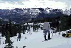
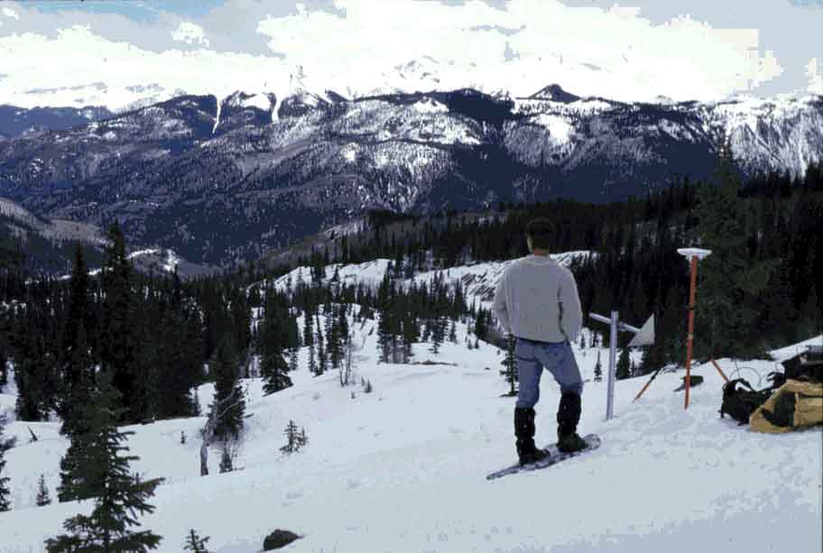
May 1999 view looking southwest down the landslide from GPS monitoring point MP5.
|
This report is preliminary and has not been reviewed for conformity with U.S. Geological Survey
editorial standards or with the North American Stratigraphic Code. Any use of trade, product, or firm names is
for descriptive purposes only and does not imply endorsement by the U.S. Government.
Open-File Report 00-101
on-line edition
2000
Abstract
Six sets of 19 GPS observations made between July 1998 and July 1999 show
that the Slumgullion landslide in southwest Colorado moved throughout the year, but that daily velocities were
highly variable on a seasonal basis. The upper part of the slide reacted more dramatically to seasonal changes
than the middle and lower parts. Maximum velocities were up to 10 times greater than minimum velocities on the
upper part of the slide and 1.8 to 1.6 times greater on the middle and lower parts of the slide. Maximum velocities
occurred between March and May on the lower part of the slide, and between May and July on the middle and upper
parts of the slide. Minimum velocities occurred between January and March for 18 of the 19 monitoring points.
Annual movements and daily velocities were smallest at the head and toe
of the landslide and largest in the central, narrowest part of the landslide. Annual combined horizontal and vertical
movement ranged from 0.15 m at the head of the slide to 7.3 m in the neck. Daily velocities ranged from <0.001
m/day to 0.024 m/day.
Introduction
The Slumgullion landslide is located about 5 km southwest of Lake
City in the San Juan mountains of southwestern Colorado (fig. 1). The active part of
the landslide is about 3.5 km long and ranges in elevation from about 2950 to 3650 m. Although the landslide has
been observed and studied since the late 1800s. (e.g., Endlich, 1876; Atwood and Mather, 1932; Crandell and Varnes,
1961; Varnes and Savage, 1996), with the exception of limited observations by Savage and Fleming, (1996), little
is known regarding the nature and magnitude of movements in response to seasonal variations and short-term meteorological
changes, and nothing is known regarding the effect of surface and subsurface water on such movements.
|

(Click to make image larger.)
Figure 1. Location map showing the active and inactive parts of the Slumgullion landslide.
|
In 1998, Brigham Young University (BYU) and the USGS began work on a 3-year
NASA-funded study of the Slumgullion landslide. The objectives of the study are to: 1) measure movement of the
entire active part of the landslide on a seasonal basis using GPS, and an airborne, interferometric capable, Synthetic
Aperture Radar and/or Scanning Microwave Altimeter remote sensing system; 2) attempt to correlate the measured
movement with observed temperature, rainfall, snow depth, and ground-and surface-water levels and pressures, 3)
evaluate the remote sensing systems for monitoring the movement of landslides by confirming a static velocity field
surrounding the landslide and by comparing remotely sensed movement data to simultaneous measurements at GPS points
and to previously measured deformation rates, and 4) develop a model for landslide deformation based on all of
the combined data. BYU is responsible for designing, building, and operating the remote sensing system(s). Current
(January, 2000) plans call for the acquisition of airborne remote sensing data beginning in the summer of 2000.
The USGS is responsible for monitoring movement using GPS, as well as monitoring hydrologic and meteorologic fluctuations
on the slide. The purpose of this report is to 1) present 6 sets of GPS observations made between July 1998 and
July 1999 and 2) describe the annual and seasonal landslide movement indicated by the observations. A preliminary
interpretation of the landslide movement is given in a separate report (Coe and others, 2000).
Methods
Installation and distribution of control points, monitoring points, and corner ceflectors
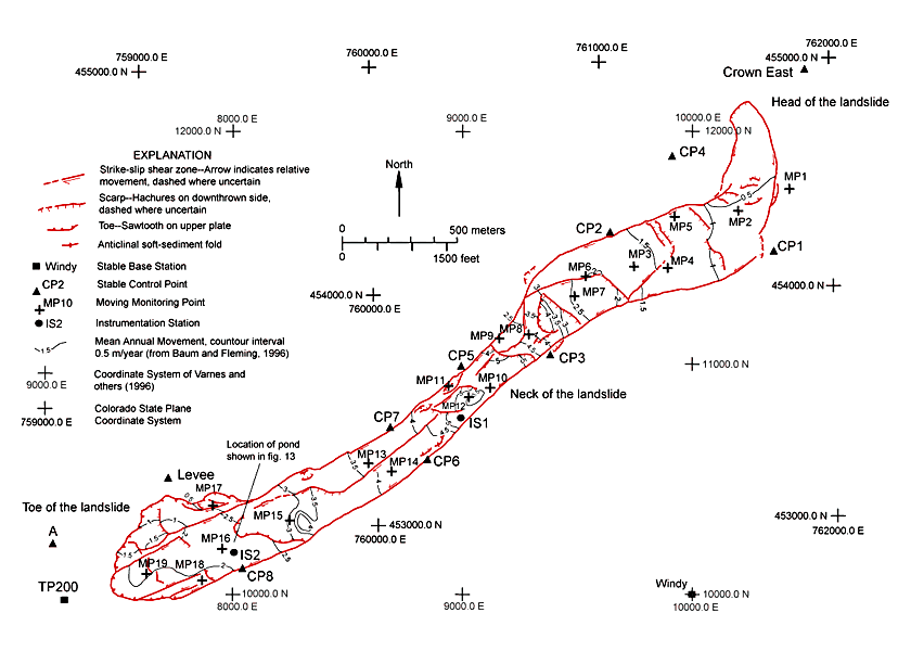
In July, 1998, 11 control points and 19 monitoring points were installed
around and on the active landslide, respectively (fig. 2). Control points were evenly
distributed in stable areas around the periphery of the slide. Control points were commonly installed on old landslide
flank ridges just outside the boundaries of the active slide. The purpose of control points is to provide a stable
reference frame in which to register remote sensing imagery to a local coordinate system. The 19 monitoring points
were evenly distributed on the active slide, but also strategically placed in relation to the main structural components
of the slide (fig.2) and with a clear view to the sky. The purpose of monitoring points
is to monitor seasonal movement of various structural components using GPS and to provide ground-truth to compare
with movements measured by remote sensing.
|
(Click to make image larger.)
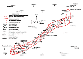
Figure 2. Active part of the Slumgullion landslide with structural elements, contours of mean annual movement,
GPS base stations, control points, and monitoring points. Modified from Baum and Fleming (1996).
|
At each control and monitoring point location, a 1.5-cm-diameter, 60-cm-long
rebar rod was hammered into the ground and an aluminum cap was attached to the end at the ground surface. A dimple
and the point name were stamped on each cap. The dimple was the location measured by GPS. At each point, a corner
reflector was installed about 1.5 m above the dimple (fig. 3). The outside corner of
each reflector was aligned so that it was plumb above the dimple and the distance from the dimple to the corner
was measured and recorded. The function of corner reflectors is to make points visible to the airborne remote sensing
system by reflecting the microwave signal directly back to the airborne sensor, creating a spike in the digital
data and a bright pixel in imagery.
|

(Click to make image larger.)
Figure 3. Installation of a corner reflector above monitoring point MP6. Photo taken in July, 1998.
|
GPS background
The following discussion of GPS surveying is summarized from Leick (1990)
and Van Sickle (1996). The primary task of GPS surveying is to measure distances between 24 Department of Defense
satellites in known orbits about 20,000 km above the earth and locations on the earth. Once distances have been
measured, coordinates of positions on the earth are calculated by triangulation. Distances are measured based on
the amount of time required for an electromagnetic GPS signal to travel from the satellites to ground-based antennas
and receivers. Antennas collect the satellite signal and convert the electromagnetic waves into electric currents
that can be recorded by the receiver.
Satellites transmit precise time and location information in three binary
codes, precise code (P code), coarse and acquisition code (C/A code), and Navigation code. The codes are transmitted
on two carrier waves that are part of the L-band of the microwave electromagnetic spectrum. The two carrier waves
have frequencies called L1 (1,575.42 Mhz, 19 cm wavelength) and L2 (1,227.60 MHz, 24 cm wavelength).
There are two GPS observables that are used to determine distances from
satellites to the ground, pseudorange and carrier phase. Pseudorange is a preliminary distance determined on the
basis of a comparison of clock information contained in the C/A and P codes with a replica of the codes generated
by the receiver. Pseudorange is used to determine approximate locations on the ground. Carrier phase is the cumulative
number of phase cycles (including the fractional part of the last cycle) of the L1 and/or L2 carrier wave signal
as measured at the receiver. Unlike pseudorange, use of the carrier phase allows for correction of atmospheric
effects and clock offsets between the satellite and receiver. Carrier phase is used for high-precision GPS surveying.
There are two main GPS surveying methods, kinematic and static surveying.
In kinematic applications, receivers are in motion during the measurement period and real-time positioning solutions
are available based on the pseudorange observables. In static applications, receivers are stationary for long-measurement
periods (generally > 30 minutes) and both pseudorange and carrier-phase data are post-processed for precise
positioning solutions. Rapid-static applications are the same as static techniques except that occupation times
are short, generally ranging from 5 to 20 minutes, and post-processing relies on code and L1 and L2 carrier phase
observations.
The type and accuracy of positioning in kinematic and static surveying is
dependent on the number of receivers available. There are two types of positioning, single point and relative.
Single-point positioning is the determination of a ground position using one receiver and observables from one
or more satellites. Single-point positioning relies on the pseudorange observable. The accuracy of the single-point
positioning increases with the number of satellites available. Relative positioning is the determination of a ground
position using two or more receivers and two or more satellites. Relative positioning allows for the elimination
of clock and atmospheric errors in the carrier-phase signal by combining simultaneous observables (referred to
as differencing in GPS terminology) from multiple receivers and satellites during post-processing. Relative positioning
determines the precise vector (baseline) between receiver positions. When the coordinates of one of the receiver
positions is known, that receiver is referred to as a base station, and the known coordinates and baseline can
be used to determine the precise coordinates of the unknown points.
In relative positioning, data is stored in the receivers and is post-processed
using computer software to calculate baselines, determine unknown coordinate positions, and estimate horizontal
and vertical errors for calculated positions. If baselines are calculated from two or more base stations, the baselines
and coordinates of unknown points can be further refined through the use of a least-squares adjustment performed
by holding the base station positions fixed while adjusting the baselines and coordinate positions of the unknown
positions.
A requirement of relative positioning is that the receivers are capable
of recording at least one of the carrier phases. Although many types of receivers are available, dual-frequency
receivers are commonly used for relative positioning because they record all GPS codes, as well as the L1 and L2
carrier phases. In addition to recording all components of the GPS signal, dual frequency receivers generally have
12 channels, which allows them to simultaneously record the signals of up to 12 satellites.
The coordinate system used by GPS is the World Geodetic System 1984 (WGS84).
The WGS84 coordinate system is based on an ellipsoidal model of the earth’s surface. Therefore, GPS receivers provide
raw positional data in WGS84 coordinates consisting of latitude, longitude, and ellipsoid height. Transformations
of latitude and longitude values into other datums, such as the North American Datum of 1983 (NAD83), followed
by projections into local coordinate systems, such as state plane systems, is accomplished through the use of software
containing conversion algorithms provided by the U.S. National Geodetic Survey (NGS). Ellipsoid heights can be
transformed into other vertical datums, such as the North American Vertical Datum of 1988 (NAVD88), by subtracting
a theoretical geoid height (see Van Sickle, 1996).
GPS observations
All control and monitoring points were surveyed using Ashtech Z-12 and Z-Surveyor,
dual-frequency receivers equipped with Ashtech geodetic or marine antennas.
Rapid-static GPS surveying with relative positioning was used for all points.
Control points were surveyed one time, in July, 1998. Current plans (January, 2000) call for control points to
be resurveyed at least one more time before the end of the project. Monitoring points were surveyed during six,
2-day GPS field campaigns. The dates of the six campaigns were as follows: July 28-29, 1998; October, 21-22, 1998;
January 5-6, 1999; March 23-24, 1999; May 11-12, 1999; and July 27-28, 1999.
Two base stations, TP200 and Windy (fig. 2), were
used for each GPS survey. Windy and TP200 consist of rebar with stamped bronze caps. Both stations were originally
installed in the early 1990s (see Varnes and others, 1996). The WGS84 positions of Windy and TP200 were determined
by a static GPS survey in May, 1997. Positions were determined using a Federal Base Network Control Station (Station
Designation S424, located near the Blue Mesa reservoir about 50 km north of Lake City) as a base station.
All GPS data were post-processed using Ashtech Precise Navigation (PNAV)
software, v. 2.4.00M. Baselines and positions were calculated from Windy and TP200 for each of the control and
monitoring points. By calculating baselines to each measured point from two base stations, a triangle was formed
with one side known (TP200 to Windy), and two sides measured (Windy to measured point and TP200 to measured point).
The measured baselines and point positions were then refined using a least-squares adjustment contained in Ashtech
PRISM software, v. 2.1. During the adjustment, the positions of Windy and TP200 were held fixed and the baselines
and positions of the measured points were adjusted. In general, positions of adjusted points did not change by
more than 1 cm in horizontal and 2 cm in vertical from the original positions as determined from GPS data alone.
In some cases, the original, unadjusted point positions as determined by
GPS alone were used as the final reported positions. These cases were the result of problems at base stations.
Most commonly, problems were encountered during winter surveys and included dead receiver batteries and settling
of tripod legs in thawing ground during daylight hours. Most problems were encountered at station Windy because
of exposure to wind and solar extremes.
After surveying, post-processing, and adjustment, coordinate positions for
all measured points were transformed into the NAD83 datum and then projected into the Colorado State Plane, southern
zone, coordinate system using PRISM software. Ellipsoid heights were transformed into NAVD88 mean sea level heights
using PRISM software and the GEOID96 model provided by the NGS. Standard errors of computed positions were derived
from the least squares adjustment, or from PNAV in cases where GPS data alone were used for final positions.
Results
Base station, control point, and monitoring point positions
Dates of observation, coordinates, and heights of the two base
stations, TP200 and Windy, as well as the eleven control points around the periphery of the landslide are given
in table 1. Dates of observation, coordinates, heights, and positional errors for all
monitoring points are given in table 2. Positional errors are given as standard errors
and are always less than or equal to 1 cm in horizontal and 1.5 cm in vertical. At all points except MP1 and MP17,
these errors are insignificant in comparison to the amount of movement that occurred between each GPS observation.
|
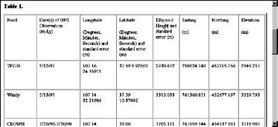
(Click to image to open Table 1.)
|
|
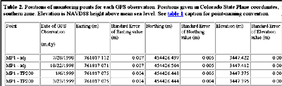
(Click to image to open Table 2.)
|
Movements and velocities of monitoring points
All monitoring points moved between each set of GPS observations (see table 3 for movement data and Appendix A for figures showing movement of each point). Total
movement (combined horizontal and vertical movement) was largely dominated by the horizontal component (see annual
combined and annual horizontal movement, table 3). In a general sense, annual horizontal
movements and average annual velocities are smallest near the head and toe of the landslide and increase to a peak
at the central, narrowest part (neck) of the landslide (fig. 4 and fig.
5). Annual horizontal movements ranged from 0.15 m at MP1 to 7.3 m at MP12 (fig. 4a). Average daily horizontal
velocities over the yearlong monitoring period ranged from <0.001 m/day at MP1 to 0.020 m/day at MP12 (fig
4b). Annual vertical movements ranged from less than 0.01 m at MP1 to 1.29 m at MP10. All points, except MP16,
moved downslope. MP16 moved upward (see Appendix, MP16).
|
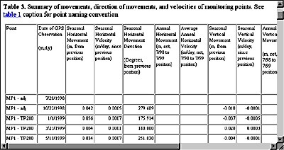
(Click to image to open Table 3.)
|
|
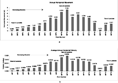
(Click to make image larger.)
Figure 4. Bar graph showing the distribution of a) annual horizontal movement and b) average daily horizontal
velocities over the year-long monitoring period.
|
Velocities of individual points varied considerably according to the season,
with minimum values ranging from 10-66 percent of maximum values (fig. 6). The largest
differences occurred at points near the head of the slide (MP1, MP2, MP5) where the seasonal minimum velocities
were 10-27 percent of the seasonal maximums. The smallest differences occurred at points in the neck of the slide
(MP9, MP10, MP12, MP11, MP14, and MP13) where the seasonal minimum velocities were 63-66 percent of the seasonal
maximums.
|

(Click to make image larger.)
Figure 5. Diagram showing cumulative horizontal movement of monitoring points. Ending dates of GPS campaigns
are shown.
|
|
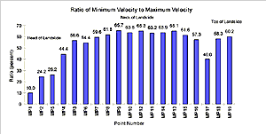
(Click to make image larger.)
Figure 6. Bar graph showing the ratio of minimum velocity to maximum velocity at each monitoring point.
|
Minimum and maximum velocities occurred at different times on different
parts of the slide (fig. 7). At 15 of the 19 monitoring points (MP1-MP15), maximum velocities
occurred between May 12 and July 28. At the remaining four points (MP16-MP19), located at the lowest elevations
near the toe of the slide, maximum velocities occurred between March 24 and May 12. Minimum velocities at all points,
except MP17, occurred between January 6 and March 24. At MP17, the minimum velocity occurred between October 22
and January 6.
|
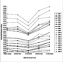
(Click to make image larger.)
Figure 7. Diagram showing daily velocities of monitoring points. Dates shown are periods between GPS observations.
|
Summary
Data presented in this report indicate that all parts of the active portion
of the Slumgullion landslide moved throughout the 1998/1999 monitoring year. Daily velocities, however, were highly
variable on a seasonal basis. Minimum velocities occurred between January and March, whereas maximum velocities
occurred between March and May on the lower part of the slide, and between May and July on the middle and upper
parts of the slide. Annual and seasonal velocities were greatest at the neck of the landslide and gradually decreased
both upslope and downslope with the lowest velocities occurring at the head and toe of the slide.
Acknowledgments
We thank Perry Hardin, Nicolas Houdré, Caroline Arnal, Manuelle Seigneur,
Graham MacDonald, Oswaldo Filho, Kathy Varnes, and Josh Ellis for their assistance with GPS surveys at various
times. We appreciate the efforts of David Arnold and his students at BYU in designing and building the corner reflectors.
Dave Kibler and Perry Hardin developed the methodology for mounting corner reflectors above control and monitoring
points. Bob Fleming and Mark Reid had helpful suggestions at the start of the project. Rex Baum had helpful suggestions
throughout the monitoring period and also reviewed this report. This study was funded by the NASA Solid Earth and
Natural Hazards research program (NRA-MTPE-1997-10), Principal Investigator, David Arnold, Brigham Young University,
Co-Investigator, Jeff Coe, USGS.
References Cited
Atwood, W.W. and Mather, K.F., 1932, Physiography and Quaternary geology of the San Juan mountains, Colorado:
U.S. Geological Survey Professional Paper 166, 176 p.
Baum, R.L. and Fleming, R.W., 1996, Kinematic studies of the Slumgullion landslide, Hinsdale County, Colorado:
in Varnes, D.J. and Savage, W.Z., eds., The Slumgullion Earth Flow: A large-scale natural laboratory, U.S.
Geological Survey Bulletin 2130, p. 9-12.
Coe, J.A., Godt, J.W., Ellis, W.L., Savage, W.Z., Savage, J.E., Powers, P.S., Varnes, D.J., and Tachker,
P., 2000, Preliminary interpretation of seasonal movement of the Slumgullion landslide as determined by GPS observations,
July 1998 - July 1999: U.S. Geological Survey Open-File Report 00-102, 25p.
Crandell and Varnes, 1961, Movement of the Slumgullion Earthflow near Lake City, Colorado, in Short
papers in the geologic and hydrologic sciences: U.S. Geological Survey Professional Paper 424-B, p. B136-B139.
Endlich, F.M., 1876, Report of F.M. Endlich, in U.S. Geological and Geographical Survey (Hayden) of the
Territories Annual Report 1974, p. 203.
Leick, A., 1990, GPS satellite surveying: Wiley and Sons, New York, 352 p.
Savage, W.Z. and Fleming, R.W., 1996, Slumgullion landslide fault creep studies, in Varnes, D.J.
and Savage, W.Z., eds., The Slumgullion Earth Flow: A large-scale natural laboratory, U.S. Geological Survey Bulletin
2130, p 73-76.
Van Sickle, J., 1996, GPS for land surveyors: Ann Arbor Press, Chelsea, Michigan, 209 p.
Varnes, D.J., Smith, W.K., Savage, W.Z., and Powers, P.S., 1996, Deformation and control surveys, Slumgullion
landslide: in Varnes, D.J. and Savage, W.Z., eds., The Slumgullion Earth Flow: A large-scale natural laboratory,
U.S. Geological Survey Bulletin 2130, p. 43-49.
Varnes, D.J. and Savage, W.Z., 1996, The Slumgullion Earth Flow: A large-scale natural laboratory, U.S. Geological
Survey Bulletin 2130, 95 p.
|
 |