Montana Bureau of Mines and Geology
Montana Tech of the University of Montana
Butte, MT 59701-8997
Telephone: (406) 496-2986
Fax: (406) 496-4451
e-mail: pkennelly@mtech.edu
Correlation of aeromagnetic and isostatic residual gravity patterns to maps of surficial geology is often the first step in making interpretations such as those noted above. This requires the overlay of potential field data with the mapped geology. Although Geographic Information System (GIS) technology makes this overlay simple, the resulting displays are often difficult to visualize, especially for users unfamiliar with potential field data.
This paper outlines a method for using GIS to create three-dimensional (3D) displays of potential field and geologic data. First, a 3D surface is built from the aeromagnetic or gravity data. Then, a layer representing geology can be draped over these surfaces, with geologic formations represented with colors.
The resulting grid for Montana has a spatial resolution of 500 meters, with each grid cell assigned a measure of the local magnetic field in nano-teslas. These values define a continuous potential field surface, much as the elevation Digital Elevation Model (DEM) grid cells define a topographic surface. Variations in the aeromagnetic potential field are due to lateral variations in content of magnetic minerals in surfical or subsurface geology, especially variations in the mineral magnetite (Telford et. al., 1976).
The isostatic residual gravity grid applies further corrections to the Bouguer gravity anomaly grid to account for lateral variations at the crust/mantle interface resulting from topography (Simpson et.al., 1986). The computation assumes an Airy model of isostacy, thus topographic highs have associated low density crustal roots to provide bouyancy, allowing them to "float" on the mantle in a manner similar to an iceberg on water. The isostatic correction used the Bouguer gravity anomaly grid, a topographic grid, and three assumptions. It assumed a crustal thickness of 30 km., a density for the crust of 2.67 g/cc, and a density contrast between crust and mantle of 0.35 g/cc.
Given these assumptions, the resulting isostatic residual gravity grid should give the best image of lateral density variations associated with surficial or near-surface geology. The isostatic residual gravity grid cells are 500 meters, with each grid cell assigned a value of the local isostatic residual gravity field in miligals (mgal). The grid cells define a continuous surface for the isostatic residual gravity field.
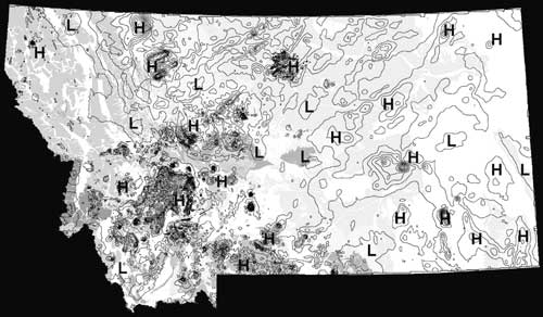
Figure 1. A geologic map of Montana overlain with aeromagnetic equipotential contours. The contour interval for the aeromagnetic data is 200 nanoteslas. |
Figure 2 is a black and white example of a color isostatic residual gravity map with a geologic formation contact overlay. This display clearly indicates gravity highs and lows, but geologic formations are difficult to visualize. Only larger geologic polygons can be labeled at this scale. Also, it is difficult to see the continuity of formations that are comprised of a number of polygons.
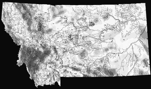
Figure 2. The isostatic residual gravity map of Montana overlain with geologic contacts. |
Once the geology has been converted to a grid, the geology can be displayed on a 3D potential field surface with ArcView and the 3D Analyst extension. To create such displays, open a 3D scene, add the geology grid theme, and use the legend editor to assign colors based on geologic formation information. Then, select "3D properties" under the "Theme" dropdown menu. In the "Assign base height by:" portion of the menu, select the radio button for "Surface", then select a potential field grid. To enhance the 3D effect, select "Properties" under the "3D Scene" dropdown menu. Then, adjust the "Vertical exaggeration factor:" until the appropriate 3D effect is achieved. These numbers are not true vertical exaggerations as horizontal units are in distance (meters) and vertical units are in nanoteslas for aeromagnetic data and miligals for gravity data. In our examples below, the vertical exaggeration factors are 30x's for the aeromagnetic data and 750x's for the isostatic residual gravity data.
Figure 3 shows a color geology map displayed in black and white on an aeromagnetic surface. The most obvious correlation is between isolated, volcanic intrusives and sharp spikes in the magnetic field. Examples can be seen in the southwest of the map, as well as in a single spike in the northwest. Other less magnetic intrusive volcanics, such as the Idaho batholith on the west-central Idaho border, have no such associated highs.

Figure 3. A geologic map of Montana draped over a 3D aeromagnetic surface. The horizontal scale is in meters and the vertical scale is in nanoteslas. The "vertical exaggeration" is 30x. |
Figure 4 shows a color geology map displayed in black and white on an isostatic residual gravity surface. This map illustrates lateral changes in density of rock formations. The narrow NNW trending Cedar Creek anticline is defined by a gravity high and adjacent lows on the western edge of Montana. A broader feature, the Sweet Grass arch, is defined by an isostatic residual gravity high in northwestern Montana. The Powder River basin in southeastern Montana is defined by a gravity low correlating to Tertiary sediments surrounded by Cretaceous rocks. As with its magnetic intensity, the Idaho batholith on the western edge of Montana has no large density variations with surrounding formations.

Figure 4. A geologic map of Montana draped over a 3D isostatic residual gravity surface. The horizontal scale is in meters and the vertical scale is in milligals. The "vertical exaggeration" is 750x. |
Aeromagnetic and isostatic residual gravity data for other states is also available from the U.S. Geological Survey. These data can be accessed from http://crustal.usgs.gov/crustal/geophysics/. To view a version of this paper with color figures, please refer to http://www.mbmg.mtech.edu/pdf/gis-dmtposter.pdf.
Harris, J.R., Viljoen, D.W., and Rencz, A.N., 1999, Integration and visualization of geoscience data, In Remote Sensing for the earth sciences(A. N. Rencz, ed.) , Vol. 3: Manual of remote sensing, (R. A. Ryerson, ed.), 3rd ed, John Wiley & Sons, Inc., New York, p. 341.
McCafferty, A.E., Bankey, V., and Brenner, K.C., 1998, Merged aeromagnetic and gravity data for Montana: A web site for distribution of gridded data and plot files: U.S. Geological Survey Open-file Report 98-333, 20 p, http://greenwood.cr.usgs.gov/pub/open-file-reports/ofr-98-0333/.
Plouff, D., 1977, Preliminary documentation for a FORTRAN program to compute gravity terrain corrections based on topography digitized on a geographic grid: U.S. Geological Survey Open-File Report 77-535, 43 p.
Ross, C. P., D. A. Andrews, and I. J. Witkind, 1955, Geologic map of Montana: Montana Bureau of Mines and Geology Geologic Map Series Geol-1, 2 sheets. Scale 1:500,000. (Out of print).
Simpson, R.W., R. C. Jachens, R.J. Blakely and R. W. Saltus, 1986, A new isostatic residual gravity map of the conterminous United States with a discussion on the significance of isostatic residual anomalies, J. Geophys. Res., 91, pp. 8348-8372.
Telford, W. M., Geldart, L. P., Sheriff, R.E., and Keys, D.A., 1976, Applied Geophysics, Cambridge University Press, New York and Melbourne, First Edition, 118p.