
|
2002
This report is preliminary and has not been reviewed for conformity with U.S. Geological Survey editorial standards or with the North American Stratigraphic Code. Any use of trade names in this publication is for descriptive purposes only and does not imply endorsement by the U.S. Government.
U.S. Department of the Interior
U.S. Geological Survey
|
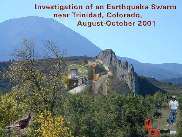
Spanish Peaks, eastern flank of the Sangre de Cristo range, near Trinidad,
Colorado
Cover design by Margo Johnson, U.S.G.S. Photo credit: Mark Meremonte and David Carver (U.S. Geological Survey) |
II. Earthquake response goals.
III. Understanding the current earthquake activity.
B. Alignment of earthquake epicenters:
C. Earthquake frequency and spatial patterns:
1. Seismograph instrumentation.
a) Data logger and Seismometer:
A swarm of 12 widely felt earthquakes occurred between August 28 and September 21, 2001, in the area west of the town of Trinidad, Colorado. The earthquakes ranged in magnitude between 2.8 and 4.6, and the largest event occurred on September 5, eight days after the initial M 3.4 event. The nearest permanent seismograph station to the swarm is about 290 km away, resulting in large uncertainties in the location and depth of these events. To better locate and characterize the earthquakes in this swarm, we deployed a total of 12 portable seismographs in the area of the swarm starting on September 6. Here we report on data from this portable network that was recorded between September 7 and October 15. During this time period, we have high-quality data from 39 earthquakes. The hypocenters of these earthquakes cluster to define a 6 km long northeast-trending fault plane that dips steeply (70-80°) to the southeast. The upper bound of well-constrained hypocenters is near 3 km depth and lower bound is near 6 km depth. Preliminary fault mechanisms suggest normal faulting with movement down to the southeast.
Significant historical earthquakes have occurred in the Trinidad region in 1966 and 1973. Reexamination of felt reports from these earthquakes suggest that the 1973 events may have occurred in the same area, and possibly on the same fault, as the 2001 swarm.
In recent years, a large volume of excess water that is produced in conjunction with coal-bed methane gas production has been returned to the subsurface in fluid disposal wells in the area of the earthquake swarm. Because of the proximity of these disposal wells to the earthquakes, local residents and officials are concerned that the fluid disposal might have triggered the earthquakes. We have evaluated the characteristics of the seismicity using criteria proposed by Davis and Frohlich (1993) as diagnostic of seismicity induced by fluid injection. We conclude that the characteristics of the seismicity and the fluid disposal process do not constitute strong evidence that the seismicity is induced by the fluid disposal, though they do not rule out this possibility.
On August 28, 2001, the first of a swarm of earthquakes occurred near Trinidad, Colorado, a small town (population approximately 10,000) near the Colorado-New Mexico border that is situated along the Santa Fe Trail and Interstate 25 (Figure 1 ).
|
Click Image for detail Figure 1. Map of the state of Colorado and surrounding region showing the location of Trinidad, Colorado, where the swarm of felt earthquakes occurred. |
Between August 28 and September 21, 2001, the U.S.
Geological Survey (USGS) National Earthquake Information Center (NEIC) recorded
and located 12
earthquakes of magnitude 2.8-4.6 in the region west of Trinidad. The largest
earthquake (M 4.6) was the fifth event in the swarm and occurred eight days
after the initial M 3.4 event (Figures 2 and 3). All of the earthquakes were widely felt in
the Trinidad area, especially in the small towns of Cokedale, Valdez, and Segundo,
which are located 10-19 km (6-12 mi) west of Trinidad (Figure 4). The felt area for the M 4.6 event extended
~32 km (20 mi) south to Raton, New Mexico, ~32 km (20 mi) north to Aquilar,
Colorado, and ~32-48 km (20-30 mi) west to Weston and Stonewall, Colorado.
|
Click Image for detail Figure 2. Catalog of the 12 felt earthquakes in the vicinity of Trinidad, Colorado reported by the USGS National Earthquakes Information Center between August 28 and September 21, 2001. |
Figure 4 shows the locations of the 12 earthquakes recorded by the NEIC. These epicenters are widely scattered in the general area 5-19 km (3-12 mi) WSW of Trinidad and show little evidence of an alignment that could indicate a causative fault. Because the nearest permanent station (Albuquerque, NM) of the United States National Seismograph Network (USNSN ) is more than 290 km (180 mi) away, the uncertainties in the location and depth of the earthquakes reported by the NEIC are large. These location uncertainties are of the order ± 10 km (6 mi), and the exact depths within the crust cannot be determined. However, NEIC officials (W. Person, pers. commun., 2001) reported that the “character of seismograms of the earthquakes implies that they occurred in the uppermost 16 km (10 mi) of the earth's crust.”
Considering the absence of close-in seismographs
to provide good location and depth control and the occurrence of five felt
events over an eight-day period, the USGS decided to install a local network
of portable digital seismographs. Figure 5 shows the location of the local seismograph
network of 12 portable digital seismographs; and Figures 6 and 7 are photographs of a typical seismograph station
in this network (see Appendix: Seismograph instrumentation, Network design,
and Network management).
|
Click Image for detail Figure 3. A plot of the earthquake magnitude of earthquakes in the Trinidad, Colorado, swarm vs. the date and approximate time of their occurrences. |
Other circumstances also contributed to USGS’s decision to respond to the Trinidad earthquake swarm. Currently coal-bed methane gas is under production west of Trinidad. The process of coal-bed methane gas extraction involves the removal of large amounts of water from the shallow coal beds and, due to environmental regulations, the excess water is returned to deeper underground layers. Thus, data from a local seismograph network might be able to shed some light on whether a relationship between the earthquake activity and the fluid disposal operation existed.
The primary focus of the Trinidad earthquake study is to record and accurately locate the earthquakes occurring in the area of the swarm. It is important to pinpoint the locations and depths of the earthquakes, that is, the earthquake hypocenters, to better understand their spatial distribution. These locations, together with other information derived from the seismograms, permit geophysicists to determine the type of faulting, fault orientation, fault mechanics, and fault dimensions. This information, in turn, can guide geologists to look for surface features above the hypocenters and signs of recent tectonic deformation or faulting.
|
Click Image for detail Figure 4. Locations of the 12 earthquakes in the Trinidad area reported by the National Earthquake Information Center that were widely scattered in the area 5-19 km (3-12 mi) WSW of Trinidad. The earthquakes were strongly felt in the small towns of Cokedale, Valdez, and Segundo, Colorado. |
In recent years, the area west of Trinidad has become the focus of extensive drilling for the production of coal-bed methane. Water from the coal-bed methane production is returned to the subsurface in disposal wells, and local citizens and officials in the Trinidad area expressed concern that the earthquakes might be somehow related to this fluid disposal. Previous cases of subsurface fluid disposal causing earthquakes have been reported elsewhere in Colorado. Earthquakes were induced by fluid injection at Rangely oil field (1960-1973), at the Rocky Mountain Arsenal (1962-1972 , Healy and others, 1966, 1968, and Herrmann and others, 1981), and at Paradox Valley (1991-present ).
[Information on investigations of induced earthquakes can be found at these links:
In Colorado’s earthquake history at least two episodes of past seismicity have occurred in the Trinidad area (Figure 8).
[Note: sensitive modern seismographs have only been in use since the early 1960’s, and widespread seismograph coverage was minimal across the U.S before 1974. Furthermore, the number and density of seismograph stations was much less in the past than it is today, especially in southern Colorado and northern New Mexico. Thus, it is important to understand that any earthquakes located in this area before 1974 have large uncertainties in their locations.]
|
Click Image for detail Figure 5. Locations of the 12 portable digital seismographs installed west-southwest of Trinidad, Colorado to monitor earthquake activity. Details of the instrument characteristics are described in the appendix. |
A widely felt magnitude 4.6 earthquake occurred on
October 2, 1966, and was felt over a 38,400 km2 (15,000 mi2)
area that extended south to Roy, New Mexico, east to Two Buttes, Colorado,
north to Pueblo, Colorado, and west to the Weston and Stonewall, Colorado. The
published location for this event, which is just northeast of Trinidad, has
an uncertainty of ±10 km (±6 mi). However, detailed analysis of this event
precludes its epicentral location and, consequently, its source area to be
anywhere else except in the region northeast of Trinidad (J. Dewey, pers. commun.,
2001). Therefore, this event is not associated with the current seismicity.
In September 1973, a swarm of six earthquakes occurred in a period of five days and was felt in and around Segundo. The two largest events had magnitudes of 3.1 and 4.2. The published locations of these two earthquakes are directly northwest of Trinidad Lake (Figure 8) but their exact locations are uncertain by at least ±10 km (±6 mi). Considering the location uncertainty and the felt report information, this historical earthquake swarm could have originated from the same source area as the current earthquake swarm.
|
Click Image for detail Figure 6. USGS technician configuring a RefTek portable digital seismograph at station BH0 using a notebook PC. |
Man-made reservoirs can potentially induce earthquakes due to reservoir loading after impoundment. Reservoir-induced seismicity has been long recognized and studied extensively.
[Visit these web sites for more information:
|
Click Image for detail Figure 7. Photograph of a Guralp CMG-40T seismometer at station BH0 being buried in a 1-foot-deep hole. Burying the seismometer improves the sensitivity of the equipment and its ability to record small-magnitude earthquakes. |
Trinidad Lake, which is located near the earthquake swarm, was designed and constructed by the U.S. Army Corps of Engineers in the 1970s and completed in 1979. Considering that the 1966 and 1973 earthquake activity occurred before Trinidad Lake impoundment, that the reservoir is significantly shallower than the depth of reservoirs that have induced seismicity elsewhere, and that the current seismic activity occurred 22 years after impoundment, the likelihood that the current swarm of earthquakes is directly related to reservoir-induced seismicity is very small. However, the design of any dam does include the assessment of the potential seismic ground motions expected, and the Trinidad Lake dam is no exception.
[See U.S. Army Corps of Engineers: for more information on earthquake design of civil works projects.]
|
Click Image for detail Figure 8. Locations of two historical earthquakes that occurred in 1973 as part of a swarm of six events recorded southwest of Trinidad, Colorado, near Trinidad Lake. The felt area for this swarm was similar to the felt area for the 2001 swarm. |
Between 1862 and the 1960s, coal mining was the dominant industry in the Trinidad area, but since the 1980’s, coal mining has been replaced by coal-bed methane gas production. Information on investigations of coal mining and petroleum and gas production induced earthquakes are listed below:
And NEIC routinely identifies and catalogs mining-induced earthquakes:
However, no such events related to either coal mining or coal-bed methane-gas production in the Trinidad area have been cataloged by the NEIC to date.
[More information on gas activities in the Trinidad area can be found at Evergreen Resources, Inc.. Click on “Projects”, then on “Raton Basin.”]
|
Click Image for detail Figure 9. Locations of the 10 fluid disposal wells managed by Evergreen Resources, Inc., in area of the 2001 earthquake swarm. These wells dispose of excess water produced during the production of coal-bed methane gas. |
The process of coal-bed methane gas extraction results in the production of large amounts of excess water. The Colorado Oil and Gas Conservation Commission’s (COGCC) rules and regulations require that some of the excess water be returned to the subsurface in disposal wells, and 10 fluid disposal wells are presently operating in the earthquake-monitored area (Figure 9). The first fluid disposal well began operating in mid-1988 and the latest well began September 4, 2001. All wells are disposing of the water at various flow rates at depths of 1.5 – 2.1 km (4,000 – 7,000 ft). At all sites but two the water is freely accepted by the target geologic formation. No other external pressure is applied except for the hydrostatic pressure of the water column itself in the borehole, so no pumping is necessary. Both sites where external pressure is applied are located in the west-southwestern part of the earthquake-monitored area near station BH0. Well head Pressures at the two sites range from 160-900 psi (COGCC, writ. commun., 2001).
[More information is available from the COGCC website: click on “Information Systems” to access the Colorado oil and gas well database. Next click on “Go to GIS online”, allow the GIS viewer plug-in to install automatically, and proceed to browse the GIS online oil and gas well database system. Use the “magnifier” to enlarge the map area west of Trinidad and, at some point, be sure to click on “well status” to show well differentiation details.]
|
Click Image for detail Figure 10. Stratigraphic column showing formation names and depths based on data from the fluid disposal well in the vicinity of station MAD. Computed depths of earthquake hypocenters are more than four thousand feet below the bottom of the disposal well. |
The region west of Trinidad lies within the Raton basin, which contains a thick section of Cretaceous and Tertiary sedimentary rocks composed of sandstone, siltstone, and shale. Contained within these sedimentary rocks are numerous coal beds that have high concentrations of methane gas. To the Northwest are the peaks of Spanish Peaks, which were formed by Tertiary volcanic and intrusive rocks. These mountains, along with large intrusive dikes that cross the Raton basin, are evidence of the geologic dynamics that have occurred in this area in the past (see Rocky Mountain Geology of south-central Colorado).
Figure 10 shows a detailed geologic column from the fluid disposal well located near seismograph station MAD. The target formation for fluid disposal at this well is the Dakota Formation, which is composed of buff conglomeratic sandstone (Johnson, 1969). The Dakota Formation has a large regional lateral extent and, in the Trinidad area, outcrops east of Trinidad along the Purgatoire River and west of Stonewall. Along the Colorado Front Range, the Dakota Formation outcrops in many places and is known as the Dakota Hogback.
Most of the other fluid disposal wells were also drilled into the Dakota except for the two wells injecting under pressure described above. The target formations of these two wells for fluid disposal are the Entrada, Dockum, and Glorietta (COGCC, writ. commun., 2001), which lie below the Dakota. Note that the formations described in Figure 10 occur at various burial depths throughout the Raton basin and therefore, occur at different depths in different wells.
The surface geology of the earthquake-monitored area comprises sedimentary rocks of sandstone, siltstone, and shale of the Raton Formation. All seismograph stations are sited on rocks of this type except for stations VAL, TKD, and DK0. These three stations are sited in the wide valleys of Picketwire Valley (VAL and CKD) and Long Canyon (DK0). The thickness of the unconsolidated material on which they are sited is unknown.
|
Click Image for detail Figure 11. Map showing epicenters of the 39 earthquakes recorded by the local seismograph network and the fluid disposal wells. The well-defined northeasterly alignment of the epicenters is strong evidence that these earthquakes are occurring on a previously unknown subsurface fault. |
Thus far we have collected data for 39 days between September 7 and October 15, 2001. We have data for 334 earthquakes that were recorded by at least two stations within a 10 second window, which averages about eight earthquakes per day. Yet, of these 334 earthquakes, those recorded by less than 5 stations cannot be located reliably. If we confine our dataset to events that were recorded by 5 or more stations within a 10 second window (see Appendix: Data analysis), then we have 39 earthquakes whose epicenters can be confidentially located (Figure 11). A plot of these epicenters reveals a northeasterly striking linear alignment positioned between the towns of Segundo and Valdez and close to the fluid disposal well near station MAD.
Figure 12 is an enlargement of the highlighted area in Figure 11 and shows two cross-sections, 12-A and 12-B. The heavy-lined box on the map outlines a 10 km x 10 km (6.25 mi x 6.25 mi) area encompassing the earthquake epicenters and the closest seismograph stations. The black arrows in the box show the view/strike direction of the cross-sections. Cross-section 12-A is a view looking N. 42º E. along the strike of the epicenters, and cross-section 12-B is an orthogonal view looking N. 48º W. Horizontal and vertical scales on both cross-sections are the same, so the boxes can be viewed as a 10 km cube. The sections include the seismograph stations to show their spatial relationship to the earthquake hypocenters.
|
Click Image for detail Figure 12. Map
showing detailed locations of earthquake epicenters in a 10 km
x 10 km box, which is an enlargement of part of figure 11. Cross-section
A (upper right panel) is a plot of the hypocenters in a view from
the southwest looking to the northeast, which is along the strike
of the fault. These hypocenters have a strike of about N. 42º E. Cross-section B (lower right panel) is a plot
of the hypocenters in a view from the southeast looking to the
northwest, which is looking at the surface of the fault plane. This view is along a bearing of |
The distribution of hypocenters in Figure 12-A suggests that they are occurring on a plane that dips steeply (~70-80°) to the southeast and strikes about N. 42º E. We have bounded the hypocenters within a parallelogram to emphasize this planar distribution. Projecting the plane of the hypocenter distribution to the surface indicates that if the hypothesized fault plane extends to the surface, then this area would be the most likely area to search for evidence of young deformation, including evidence of a surface fault.
Figure 12-B is a view of the earthquakes along the hypothesized fault plane. Similar to 12-A, we have emphasized the distribution of earthquakes within a shaded ellipse. (The two shallowest hypocenters are not included in this plot because they have large uncertainties in their depth estimates, which we discuss below.) The distribution of events in this elliptical region is not uniform; more events are located toward the edge of the region than the center. Further, there seems to be two distinct groupings in the distribution. Most of the hypocenters in the upper-right of the elliptical region occur at depths shallower than 4.0 km (13,200 ft), whereas in the lower-left, most hypocenters occur deeper than 4.5 km (14,800 ft). In map view, the northeastern earthquakes correlate with the upper-right distribution of hypocenters and the southwestern earthquakes correlate with the lower-left distribution.
|
Click Image for detail Figure 13. Catalog of the 39 earthquakes located by the local seismograph network divided into five, color-coded time periods. The table also shows the dates when seismograph stations began operation. |
The 39 earthquakes shown in Figure 13 are divided into five time periods between September 7 and October 15. The catalog also shows the dates when seismograph stations began operation. Figures 14, 15, 16, 17, and 18 display the seismicity of each time period and are subsets of the data shown in Figure 12. All figures are in the same formats as Figure 12. . Each time interval is one-week long, except for period 1, which is 11 days long. The earthquakes in each time period are color-coded to help relate the events to the information plotted in Figures 14-18. In addition to color-coding the earthquakes for each time period, Figures 14-18 show the spatial relationship of earthquakes in each period to the entire earthquake series, which are gray, enclosed circles.
A comparison of the number of earthquakes recorded
within each time period provides insight into changes in the rate of seismicity
with time. Our record of events during the first period may be incomplete
because, at that time, there were no stations closer than about 6.5 km (4 mi)
to the center of seismicity; and stations BUR and RG0 were not installed until
after September 13, that is, a week after the initial installation of the local
network (see Appendix: Network design). During the second time period, an
average of about two earthquakes occurred each day (Figure 13), whereas this rate declines to less
than one event per day in period four and about one event every two days in
period five. Yet, the rate in period three was similar to the rate in period
five. Overall, the frequency of earthquakes decreased with time but additional
data from later time periods after October 15 will better substantiate this
observation.
|
Click Image for detail Figure 14. Plot of seismicity (red dots) during the first 11 days of operation of the portable network. Earthquakes of the entire series are shown by gray dots. |
|
Click Image for detail Figure 15. Plot of seismicity (orange dots) during the next 7 days of operation of the portable network. Earthquakes of the entire series are shown by gray dots. |
Comparing the earthquake locations in Figures 14-18 one can identify spatial patterns in the seismicity. Of the five periods, only the second and fourth periods show a pattern best. During the second period (Figure 15), most earthquakes were located at depths greater than 4 km (13,200 ft), whereas during the fourth period, all the seismicity is shallower that 4 km (Figure 17). In map view, earthquakes in the second time period were concentrated in the southwestern part of the epicentral area and then, in the fourth period, solely concentrated in the northeastern part. This pattern suggests that the seismicity occurs in clusters above and below some arbitrary boundary that expresses itself in both map and cross-section views. Most events during the first period (Figure 14) have large uncertainties in their earthquake depths (see section D. “Earthquake depth errors” below) and, therefore, we are unable to interpret the hypocenter distribution. Spatial patterns during the third and fifth periods (Figures 16 and 18) are difficult to recognize since few earthquakes occurred in these intervals.
|
Click Image for detail Figure 16. Plot of seismicity (dark blue dots) during the next 7 days of operation of the portable network. Earthquakes of the entire series are shown by gray dots. |
Click Image for detail Figure 17. Plot of seismicity (light blue dots) during the next 7 days of operation of the portable network. Earthquakes of the entire series are shown by gray dots. |
|
Click Image for detail Figure 18. Plot of seismicity (yellow dots) during the next 7 days of operation of the portable network. Earthquakes of the entire series are shown by gray dots. |
|
To better characterize the quality of our earthquake depths, we organized our data into three vertical error (Ez) categories:
1) Ez < ±1.5 km (Ez < ±5,000 ft); green symbols
2) ±1.5 £ Ez < ±2.5 km (±5,000 £ Ez < ±8,250 ft); yellow symbols
3) Ez ³ ±2.5 km (Ez ³ ±8,250 ft); red symbols
|
Click Image for detail
 Figure 19. Estimated vertical errors of the earthquake hypocenters divided into three categories; red, yellow, and green; see figure for details. |
Figure 19 shows the estimated vertical errors of the earthquake hypocenters. Most hypocenters have vertical errors of less than ±1.5 km (±5,000 ft) and we are confident that these are accurate (see Appendix: Data analysis). A couple of hypocenters have vertical errors in the red category and several have errors in the yellow category. The earthquakes that have vertical errors in the red and yellow categories occurred at the beginning of the recording period when there was a limited number of stations in the network and none directly above the earthquakes to constrain the depths. Better constraints on earthquake depths were not achieved until stations BUR and RGO were installed to the north and south of the epicentral area on September 13 and 17, respectively (Figures 11 and 13); and stations VZO, MAD, and VAL were not installed in the epicentral area until after September 24. Only hypocenters satisfying the vertical depth green category were used in the following data analysis.
Two significant observations are clearly defined by the hypocenters in Figure 20, which is a summation of Figures 13-19 and includes the closest fluid disposal wells. The first is a steep fault plane that dips approximately 70-80º to the southeast and whose probable upper bound is near 3 km (10,000 ft) depth and lower bound is near 6 km (19,800 ft) depth. Second, two areas of concentrated activity, emphasized by ellipses in Figure 20-B, are evident within the fault plane. These areas suggest that the earthquakes occurred in clusters rather than randomly throughout the fault plane. In map view, these clusters correlate with the northeastern and southwestern regions of the fault. These two clusters may bound that part of the fault plane ruptured during one or more of the initial 12 earthquakes reported by the NEIC and its extent. Laterally, the earthquakes are bounded by Burro Canyon to the north and by the southern edge of Picketwire Valley to the south, a length of about 6 km (4 mi).
|
Click Image for detail
 Figure 20. Summary of information described in Figures 13-19 showing significant observations of this investigation.Map (left panel) shows location for well-located earthquakes (red dots), seismograph stations, and fluid disposal wells.Cross-sections (right panels) show plots of these data in views toward the northeast (upper right panel) and toward the northwest (lower right panel). |
The initial earthquakes in the Trinidad swarm
were located by the NEIC and, the epicenters were widely scattered (Figure
4). Following installation of the local portable digital network, a magnitude
3.4 earthquake occurred (Figure 21, 9/21/2001
19:10:59.76 ) that was recorded by both the local and national
networks. Using this earthquake as a master event enabled us to calculate
timing correction factors for each of the national network stations, and, then
we applied these correction factors to relocate the other reported earthquakes. We
still had limited control on the depths of these events, so we fixed their
depths at 5 km (16,500 ft). Figure 21 (left) shows
the original NEIC locations in blue, and Figure 21 (right) shows the relocations
in blue as well. In both maps, the earthquake shown with a yellow symbol is
the master event, and the red symbols show later earthquakes that were located
by the local network. The relocated events cluster in the area of the seismicity
recorded by the portable network, which suggests that those events initially
recorded by the NEIC likely occurred on the same fault that we define using
data from the portable instruments.
One aspect of this study is to explore the possibility that the earthquakes might be induced by water injection associated with coal-bed methane production. Conceivably, very accurate hypocenter locations alone might have provided a basis for accepting or rejecting this hypothesis, but this is not the case with the hypocenters obtained in the present study. For instance, if the hypocenters were concentrated at mid-crustal depths of 10-15 km (6-9 mi) or at substantial lateral distance from any well, this would constitute strong evidence against induced seismicity. Conversely, clusters of hypocenters at shallow depths directly beneath more than one of the wells would by themselves be strong evidence in favor of induced seismicity (Healy and others, 1968). However, although our hypocenter locations are accurate (see Appendix: Data analysis), their locations by themselves do not argue strongly for or against the induced seismicity hypothesis.
|
Click Image for detail
 Figure 21. Maps showing relocation of the original 12 earthquakes reported by the National Earthquake Information Center (NEIC) and the master event used in the calculations.Map on the left shows the initial widely scattered NEIC earthquake locations. Map on the right shows the relocated NEIC events and the 39 earthquakes located by the local seismograph network. |
To assess the seismicity at Trinidad with respect to characteristics of seismicity induced by fluid injection worldwide, we consider the Trinidad observations in terms of seven questions posed by Davis and Frohlich (1993). For a given set of earthquakes, Davis and Frohlich (1993) consider that four or more "yes" answers to their questions as suggestive but "incomplete or conflicting evidence" for induced seismicity, and they consider five or more "yes" answers to be "strong" evidence. We find (below) that only three of the questions can be answered "yes" or "tentative yes".
The questions of Davis and Frohlich (1993) are based on the perspective that a given set of earthquakes is assumed to be not induced until a convincing case can be made that it is induced. This perspective is driven by the fact that the vast majority of earthquakes are natural, and it is a perspective that helps counteract the human tendency to see cultural causes behind unusual coincidences. It is important to emphasize, however, that the fact that the data do not make a strong case for the earthquakes being induced does not imply that the data do make a strong case against the earthquakes being induced. Davis and Frohlich (1993) note, moreover, that any set of answers to their questions "is open to revision if new information or evidence becomes available." The questions nonetheless provide a useful framework to examine the diverse set of clues that may point to a suite of earthquakes having been induced by fluid injection, and the "profile" of answers to these questions provides a measure of the similarity of a given earthquake sequence to well-documented cases of injection-induced seismicity worldwide.
Question 1 (Background Seismicity): Are these events the first known earthquakes of this character in the region? For Trinidad, the answer to this question is "no". A sequence of earthquakes in 1973 was located close to the 2001 source, perhaps coincident with it.
Question 2 (Temporal Correlation): Is there a clear correlation between the time of injection and the times of seismic activity? The answer to this question for the Trinidad earthquakes is a tentative "no?". To answer this question, we consider the possibility that the earthquakes were induced by water injected into the well that is nearest station MAD (Figure 20). Water has been injected into this well since April 2000 (Shirley, 2001), but most of the earthquake activity was concentrated in a period of several weeks (August 28 – September 21, 2001) more than a year after injection began. Earthquake activity has subsequently (to the date of this writing) subsided, although fluid injection continues unchanged (COGCC; writ. commun., 2001). The examples cited by Davis and Frohlich (1993) indicate that they do not consider the onset of seismicity after a year of injection to be a "clear" temporal correlation between injection and seismicity. We consider the answer to this question to be tentative, however, because the three months that (as of this writing) have elapsed since the August/September period of seismicity are not sufficiently long to conclude that the earthquake source region has entered another period of multi-decade quiescence.
Question 3a (Spatial Correlation): Are epicenters near the wells? For Trinidad, the answer to this question is "yes".
Question 3b (Spatial Correlation): Do some earthquakes occur at depths comparable to the depth of injection? For Trinidad, the answer to this question is a tentative "yes?" The most reliably located of the Trinidad earthquakes occur at least 1.6 km (5,280 ft) deeper than the depth of injection, but Davis and Frohlich (1993) considered, for another sequence of earthquakes, that "3 km (10,000 ft) deeper" corresponded to a tentative "yes?". This answer is reasonable when we consider that the focal-depth uncertainties are of the order ±1.5 km (±5,000 ft).
Question 3c (Local Geology): If some earthquakes occur away from wells, are there known geologic structures that may channel fluid flow to the sites of the earthquakes? We consider the answer to this question to be a tentative "yes." There is some evidence in geophysical and topographic data (e.g., V. Matthews, pers. commun. to Shirley, 2001) for a northeast-trending geologic structure that passes close to the injection well near MAD and might be considered a candidate for a structure that would channel fluid flow, but neither the geologic nor hydrologic characteristics of the structure have been determined.
Question 4a (Injection Practices): Are changes in fluid pressure sufficient to encourage seismic or aseismic failure at the bottom of the well?. In most well-documented cases of injection-induced seismicity, water is introduced into geologic formations under pressure (e.g., Davis and Frohlich, 1993. In the case of Trinidad earthquakes, water is introduced via the well near MAD into geologic formations under only the force of gravity (Shirley, 2001). Our understanding is that the water is easily accepted into the formation into which it is injected (e.g., Shirley, 2001), which would imply that fluid pressure at the bottom of the well is little changed by the injection of water into the well. On this basis, we judge that the answer to this question is a tentative "no?".
Question 4b (Injection Practices): Are changes in fluid pressure sufficient to encourage seismic or aseismic failure at the hypocentral locations? As noted by Davis and Frohlich (1993), answering this question requires a model of the hydrologic system. The authors of the present report do not have the expertise in ground-water hydrology to develop such a model for the region of the Trinidad earthquakes. Moreover, we are not able to assess if there is a mechanism, well-documented scientifically and consistent with the known geology of the earthquake area, by which injection of water under the force of gravity would cause changes in fluid pressure at depths of the Trinidad sequence hypocenters sufficient to induce fault failure. We are therefore unable to answer this question.
As stated above, we have three "yes" or "yes?" answers to the questions of Davis and Frohlich (1993). The characteristics of the Trinidad sequence summarized by the answers to the above questions do not rule out the possibility of the Trinidad earthquakes being induced, but neither do they make a strong case for the Trinidad shocks being induced.
From a seismic hazard perspective, the most important implication of the earthquakes being induced would be that the earthquake activity would probably continue at the Trinidad site for a period of years as long as injection continues at its current level at the well near station MAD. If the earthquakes are naturally occurring, we would expect the level of seismicity to generally subside, although it would not be unusual to have this general subsidence of activity punctuated by occasional delayed aftershocks or bursts of aftershocks. These inferences are qualitative judgments, based on typical (but not invariable) behavior of apparently similar bursts of natural and induced earthquake activity elsewhere in the world.
The upper-crustal focal depths of the Trinidad swarm (in the upper 6 km, 19,800 ft, of the earth's crust) may have seismic hazards implications in the long-term if the earthquakes are natural. Such shallow-depth earthquakes tend to produce more intense shaking at communities close to the epicenter (within several kilometers) than do earthquakes of similar magnitude at mid-crustal depths of 10-15 km (6-9 mi). Natural earthquakes with similar shallow depths have been observed at some other locations of the Southern Rocky Mountains. An example is the M 4.6 Dulce, New Mexico, earthquake of January 23, 1966, (Herrmann and others, 1980), which is inferred to have had a source depth of about 3 km (10,000 ft). The locations of the Trinidad earthquakes support the idea that such shallow-depth earthquakes may be a characteristic mode of seismicity in the Southern Rocky Mountains.
Other seismic hazards implications of the earthquake swarm do not depend in an obvious way on whether the earthquake was induced or natural. We know from the historical record that the Trinidad area occasionally experiences natural earthquakes; so demonstrating that the 2001 earthquakes were induced would not negate the possibility of damaging natural earthquakes in the area.
Three water disposal wells in the general epicentral area bottom in the Dakota Formation, which has a wide regional lateral extent in the Raton basin and throughout the west-central U.S. If the water being supplied to this formation spreads laterally and if the fault plane extends upward to the depth of the Dakota Formation at 1.4-1.2 km (4500-4000 ft), then this recharge water may be capable of changing the hydrologic conditions along the fault and become a contributing factor in inducing the swarm. Yet, as noted previously, the injected water is easily accepted into the formation suggesting that the fluid pressure at the bottom of the well is little changed. Therefore, although there is a general spatial relation between the location of the events and some of the disposal wells, we do not have any firm evidence of a direct relationship between the fluid disposal and the earthquake swarm.
Based on our analysis, we hypothesize that the M 4.6 event of September 5, 2001, ruptured much of the shaded elliptical region outlined in Figure 20-B and subsequent aftershocks have been occurring in and around the perimeter of this rupture area. The two areas of enhanced activity, enclosed by the smaller ellipses in both map and cross-section views (Figure 20), may represent the northeastern end of the rupture extending upwards to about 4-3 km (13,200-10,000 ft) depth and the southwestern end of the fault extending downwards to 6 km (19,800 ft) depth. These areas may be where stress on the fault increased around the boundary of the M 4.6 rupture, and ensuing smaller magnitude earthquakes are continuing to take place responding to equilibrium forces within the fault.
Hypocenters from the local Trinidad network show that the recent sequence of earthquakes occurred on a previously unknown fault located at 3 km to 6 km (10,000 - 19,800 ft) below the surface. The northeast strike of the causative fault is important information because it indicates that similarly oriented faults at other locations of the Trinidad region may also be favorably oriented to slip in the current tectonic stress field, but this is true whether or not the earthquakes are natural. The seismologically-identified fault system on which the recent earthquakes have occurred deserves more study to assess its geologic characteristics, its history of past displacement, and to determine if the fault extends to depths shallower than 3 km, which is the upper limit of the well-constrained hypocenters.
Preliminary single-event focal mechanisms calculated for the 39 local earthquakes are poorly constrained due to sparse coverage of the focal sphere. However, both the composite mechanism (Figure 22) of the 39 earthquakes and the Harvard CMT (Centroid-Moment Tensor) for the M 4.6 event of September 5, 2001, concur that primary movement is normal dip-slip. Thus, the fault movement is believed to be normal, down to the southeast with possibly a small component of left lateral strike-slip.
|
Click Image for detail
 Figure 22. Plots of focal mechanism solutions determined for the M 4.6 earthquake of September 5, 2001. The left solution was determined by the Harvard Seismology: Centroid-Moment Tensor Project. The right solution is a composite focal mechanism determined from P-wave first motions of 39 earthquakes recorded by the local seismograph network using the program FPFIT (Reasonberg and Oppenheimer, 1985). Both solutions characterize slip as dominantly normal but the composite also shows a small component of left lateral strike-slip. |
This earthquake study is being conducted in collaboration
with the Colorado State Geological Survey. We thank the Colorado Gas and Oil
Conservation Commission for sharing information on the water disposal wells
and contributing Figure 13. We also thank Evergreen
Resources, Inc., for allowing access to their owned or leased lands to
accommodate our portable digital seismograph and for cooperating with this
earthquake study. If it was not for the untiring efforts of Mr. Ken Torres
(Las Animas County Commissioner) and Mr. Vince Vigil (building inspector for
Las Animas County Planning Commission), we would still be looking for sites
in some unpopulated canyon or traveling down another dead end road. We thank
the many property owners who kindly offered their assistance and services,
and allowed us to site our portable digital seismographs on their property. Their
trust in our work and integrity is greatly appreciated. Charles Pillmore (USGS
emeritus) provided us with initial topographic, geologic, and logistical information
to help us identify potential seismograph station locations. The base maps
used in the Figures are attributed to the excellent work of John Michael and
John Kosovich, both of the USGS. And, finally, we thank Steve Harmsen for
his thorough and informative review.
Colorado Oil and Gas Conservation Commission, written communication, 2001, 1120 Lincoln Street, Suite 801 Denver, Colorado 80203
Davis, S.D., and Frohlich, C., 1993, Did (or will) fluid injection cause earthquakes? - Criteria for a rational assessment, Seismological Research Letters, v. 64, p. 207-224.
Evergreen Resources, Inc., written communication, 2001, 1401 17th Street, Suite 1200, Denver, CO 80202.
Healy, J.H., Jackson, W.H., and Van Schaack, J.R., 1966, Microseismicity studies at the site of the Denver earthquakes (part 5) in Geophysical and geological investigations relating to earthquakes in the Denver area, Colorado, U.S. Geological Survey Open-File Report, March 22, 1966, 19 p.
Healy, J.H., Rubey, W.W., Griggs, D.T., and Raleigh, C.B., 1968, The Denver earthquakes, science, v.161, no. 3848, p. 1301-1310.
Herrmann, R.B., Dewey, J.W., and Park, S.-K., 1980, The Dulce, New Mexico, earthquake of 23 January 1966, Bulletin of the Seismological Society of America, v. 70, no. 6, p. 2171-2183.
Herrmann, R.B., Park, S.-K., and Wang, C.-Y., 1981, The Denver Earthquakes of 1967-1968, Bulletin of the Seismological Society of America, v. 71, no. 3, p. 731-745.
Johnson, Ross B., 1969, Geologic map of the Trinidad quadrangle south-central Colorado: U.S. Geological Survey, Geological Investigations Map I-588, scale 1:250,000.
Lahr, J.C., 1999, HYPOELLIPSE: A computer program for determining local earthquake hypocentral parameters, magnitude, and first-motion pattern (Y2K compliant version), version 1.0: U.S. Geological Survey Open-File Report 99-23, paper and on-line editions, 116 p.
Reasonberg, P. and Oppenheimer, D., 1985, FPFIT, FPPLOT, and FPPAGE: Fortran computer programs for calculating and displaying earthquake fault-plane solutions: U.S. Geological Survey Open-File Report 85-739, 47 p.
Shirley, K., 2001, Colorado quakes cause concern, American Association of Petroleum Geologists Explorer, v. 22, n. 12, p. 6,10,11, and 17.
Two types of common portable digital data loggers are being used for this study. One type, manufactured by Refraction Technology, Inc (RefTek), is a 3- or 6-channel, 24-bit digital recorder with a hard disk and GPS receiver/clock – model 72A- 08. The other type, manufactured by Kinemetrics Inc (K2), is a 3- or 6-channel, 19-bit digital recorder with PCMCIA storage cards and GPS receiver/clock – model K2. Figure 5, shows the locations of each type of data logger. The up-pointing triangle symbol denotes the RefTek while the down-pointing triangle denotes the K2.
Four types of seismometers are being used in the network. Most RefTek stations have CMG-40T broadband seismometers that record frequencies between 0.05 – 50 Hz. One RefTek station, BH0, has a Mark Products L22 seismometer, which is a short-period sensor capable of recording frequencies from 0.5 Hz and higher depending on the data-logger recording configuration. The other two types of seismometers are accelerometers that record strong motion, that is, ground motion strong enough to cause damage. These instruments, both manufactured by Kinemetrics, are the FBA-23 and the Episensor ES-T accelerometers. RefTek station, RG0, is using the FBA-23 while all of the K2 stations are using the Episensor ES-T.
Accurate timing between the portable seismographs is critical because precise earthquake locations depend on knowing the time that the P- and S-wave from earthquakes arrive at each station. These arrival times are mathematically inverted to determine when the earthquake occurred and to compute the earthquake’s latitude, longitude, and depth (Lahr, 1999). Both loggers utilize GPS (Global Positioning System) receiver/clocks to time stamp the digital data. The GPS clocks continuously receive a time signal from one or more orbiting geo-stationary satellites as a reference and compared to the time signal of a data logger’s internal clock. If a time difference exists, then the internal clock is adjusted, and the correction is written into a log file. Nominally, the timing error of an internal clock is less than 1 ms (0.001 sec), however, since the digital recording instrument logs time comparison differences, the log can be used to apply clock corrections to the data.
The instrument response files for the digital data loggers and the seismometers are available at the Geologic Hazards Website.
Our primary objective of this study was to obtain accurate information on the location, depth, and characteristics of the earthquakes. To accomplish this, we initially installed seven portable digital seismographs in an array that roughly surrounded the epicentral area as defined by the locations reported by NEIC (Figure 2). Since the NEIC locations had uncertainties on the order of ±10 km (6 mi) and because the strongest felt reports were from the towns of Segundo and Valdez, which are 19 km (12 mi) west of Trinidad, Colorado, we centered our network on these towns. The average distance between stations was based on the overall scatter of the NEIC locations, but specific locations were influenced by the density of homes in the surrounding region. To expedite and simplify our installation, we attempted to locate stations at sites where we had access to AC power, but since many canyons in the area are not populated, we needed batteries and solar panels in some places. Figure 5 shows the distribution of the 12 portable seismographs in our network.
The first stations in the network were installed by September 8, 2001 and included stations TK0, PD0, TKD, PT0, and BH0 on the perimeter and CKD and DK0 in the interior. As we began to more accurately define the earthquake epicentral area, we installed additional stations to provide better azimuth and depth control of the earthquakes (Figure 11). Our initial locations indicated that the earthquakes were located about 8 km (5 mi) directly west of Cokedale and north of Valdez, so we installed stations BUR on September 13 and RG0 on September 17 to control the locations in the north-south direction. On September 25 and 26 we installed stations VZ0 and MAD to better constrain the depths of the earthquakes. Having these stations directly above the earthquakes greatly improved our ability to estimate the depth of the events. Lastly, on October 11, we installed station VAL for better depth control on the events near the southwestern edge of the source area.
Once the network was fully operational, we systematically serviced the stations to verify their operations and to retrieve data. A few days after each station was installed, we revisited it in order to: 1) verify that the data logger was operating; 2) verify that the data logger configuration was suitable for the expected magnitude range, and 3) verify that the data logger configuration could accommodate the existing ambient background noise from manmade or natural sources. When we were satisfied with the station’s operations, we then retrieved the recorded data. When we were confident that stations were operating satisfactorily, we only visited them as frequently as needed to retrieve data.
Data from all stations was first sorted into chronological order, and an algorithm organized them into individual events. These events were then reviewed by an analyst to determine which events are earthquakes where the resulting dataset was used for all subsequent analysis. For this study, we determined that a minimum of five stations was necessary to compute a well-constrained location for individual earthquakes.
This determination was based on: 1) the final distribution of stations relative to the earthquake epicenters and 2) the distance from the epicenters to the nearest station relative to the calculated earthquake focal depths. The most accurate earthquake locations are derived from stations that are evenly distributed around the epicenters, which provides even azimuth control. However, topography, demographics, and instrumentation availability limit this distribution. For good depth control, it is important to have at least one station within one to two focal depths of the event. For this earthquake study, the depths ranged between about 3 and 6 km (10,000 to 20,000 ft), we attempted to establish our array to have stations within 3 km of individual earthquakes
The P- and S-arrival times were measured at each station for events recorded by five or more stations, and we located each earthquake using the program HYPOELLIPSE (Lahr, 1999) using a velocity model containing four layers over a half-space. Velocities in the model are:
Depth to top of layer (km) P-phase Velocity of layer (km/sec)
0.0 4.0
1.8 4.9
3.0 5.8
20.0 6.9
40.0 8.0
Precise determination of earthquake hypocenters (especially depths) depends on an accurate model of seismic velocities as a function of depth. For the upper crust, we used a three-layer velocity model consisting of a top layer of Tertiary and Cretaceous sedimentary rocks about 2 km thick, a layer of older Permian and Pennsylvanian sedimentary rock about 1 km thick, and a layer of Precambrian basement (crystalline rock) starting at a depth of 3 km (10,000 ft). The depth to basement model was based on the estimate in an unpublished map by Ogden Tweto (P. Sims, writ. commun., 2001). A P-wave velocity of 4.0 km/sec (2.5 mi/sec) was assigned to the top layer, largely constrained by the stacking velocities from reflection surveys in the region done by Evergreen Resources, Inc. (writ. commun., 2001). This velocity is typical for shallow well-consolidated sedimentary rock. A P-wave velocity of 4.9 km/sec (3.1 mi/sec) was used for the second layer, based on the velocity of similar rock at the Rocky Mountain Arsenal measured from a borehole (Healy and others., 1966). The Precambrian basement rock was assigned a P-wave velocity of 5.8 km/sec (3.6 mi/sec), again using values for this rock type measured at the Arsenal. S-wave arrival times were also used for all hypocentral determinations.
An average Vp/Vs ratio of 1.68 was determined from these data by the program HYPOELLIPSE and was used to compute S-phase travel times. No station travel-time corrections were used. The average RMS residual for all 39 events located by the local network is 0.038.
Different types of analyses on these data can determine geophysical properties of the earthquakes and other earthquake effects such as fault characteristics, magnitude, and site response. However, at this time, we are focusing our effort on determining the spatial distribution of the hypocenters.
The earthquake data and the P-wave and S-wave arrival time picks are available at the Geologic Hazards Website.
| AccessibilityFOIAPrivacyPolicies and Notices | |
| |
|


