
Digital Mapping Techniques '04— Workshop Proceedings
U.S. Geological Survey Open-File
Report 2004–1451
Conversion of Surficial Geologic Maps to Digital Format in the Seacoast Region of New Hampshire
129 Hazen Drive, PO Box 95, Concord, NH 03302-0095; Telephone: (603) 271-4087;
Fax: (603) 271-3305; e-mail: dbennett@des.state.nh.us
ABSTRACT
Over the past 20 years the Seacoast region of New Hampshire has experienced population growth that far exceeds other parts of the state. Figure 1 (Sundquist, 2000) illustrates population trends and projected growth for the state of New Hampshire. This increased population means more homes, buildings, pavement, and other impervious surfaces, which ultimately affect groundwater recharge. Serious questions have been raised about the sustainability of groundwater resources, as demand for the resource continues to rise, whereas groundwater recharge is most likely decreasing.
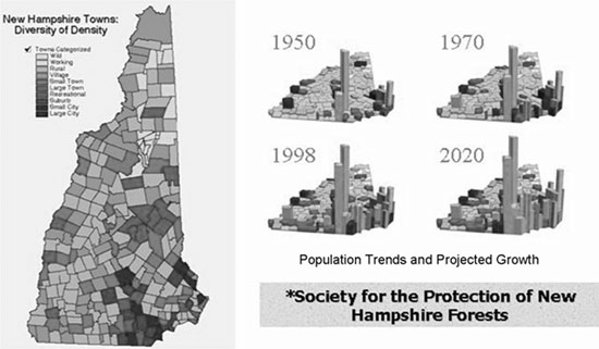 |
Figure 1. Population trends and projected growth for the state of New Hampshire. |
The New Hampshire Geological Survey (NHGS), in cooperation with the New Hampshire Department of Environmental Services (NHDES), New Hampshire Office of Energy and Planning (NHOEP), and the U.S. Geological Survey New Hampshire/Vermont district (USGS), have entered into an agreement to estimate the availability of groundwater resources at a regional scale in the Piscataqua River / Coastal drainage basin. The goal of the project is to provide southeastern New Hampshire communities with the necessary tools to make informed water resource decisions.
The thickness and distribution of surficial materials play an integral role in determining groundwater recharge, storage, and availability. Therefore, a better understanding of surficial deposits in the region is essential in order to make accurate availability estimates. NHGS has focused its mapping efforts to complete surficial mapping in the few remaining unmapped quadrangles in the area, and to convert existing maps to digital format (Figure 2).
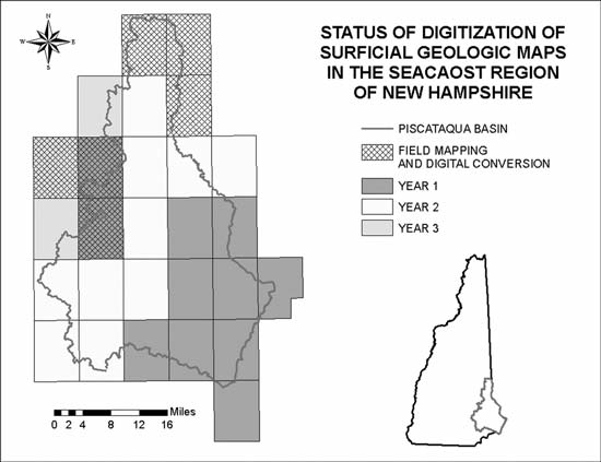 |
Figure 2. Status of surficial mapping in relation to the Seacoast project area. |
Over a three-year period the NHGS will be converting twenty-one published surficial geologic maps to digital format, as well as mapping and digitizing six new surficial geologic maps. In year one (2003), the NHGS converted the following 7.5-minute quadrangles to digital format: Dover East (Larson and Goldsmith, 1989), Dover West (Koteff and others, 1989b), Exeter (Goldsmith, 2001), Hampton (Koteff and others, 1989a), Kingston (Koteff and Moore, 1994), Kittery (Larson, 1992), Newburyport East (Koteff and others, 1989a), Newmarket (Delcore and Koteff, 1989), and Portsmouth (Larson, 1992). The Northwood (Brooks, 2004) and Parker Mountain (Koteff, 2004) quadrangles were mapped as well as digitized. In year two (2004), the NHGS digitized the following thirteen quadrangles: Baxter Lake (Goldsmith, 1993), Barrington (Goldsmith, 1990a), Candia (Gephart, 1985a), Derry (Gephart, 1985b), Epping (Goldsmith, 1990b), Farmington (Goldsmith, 1994), Mount Pawtuckaway (Goldsmith, 1997), Rochester (Koteff, 1991), Sandown (Gephart, 1987), and Somersworth (Koteff, 1991). Three new surficial mapping projects that will include digitization will be conducted in year two: Sanbornville, Great East Lake, and Milton. In year three (2005), the NHGS will digitize the remaining quadrangles covering the Piscataqua River / Coastal drainage basin: Alton (Goldsmith, 1995) and Gossville (Goldsmith, 1998). The Pittsfield quadrangle will be mapped and digitized during year three.
LOCATION AND GEOLOGIC SETTING
The Seacoast region of New Hampshire contains a complex system of sand and gravel deposits of mostly glaciomarine origin, silty facies of the glaciomarine Presumpscot Formation, glaciolacustrine and glaciofluvial deposits, at least two ages of glacial till, and locally thick eolian deposits. Glacial cover exceeds 90 percent in most areas. Tills average 15 feet in thickness but in drumlins can exceed 100 feet. There are two distinct types of till in the region. The upper or ablation till (late Wisconsinan age) is fairly sandy and slightly weathered. Till found within the drumlins (Illinoian age) is more compact and silty, and is deeply oxidized. Deltaic deposits can be as much as 150 feet thick. Most of the sand and gravel deposits in this region have been extracted, but very sizeable amounts remain. The bedrock of the region, which is the source rock for the glacial deposits, consists of metasandstone, phyllite, schist, gneiss, and granite.
APPROACH FOR CONVERTING MAPS TO DIGITAL FORMAT
The conversion of paper maps to digital format presents numerous challenges that are unique in nature. In order to develop a useful and seamless dataset, criteria for map standards, data organization, and attribution need to be established. NHGS utilized the ArcInfo coverage datamodel and organized the surficial units and textures into region subclasses (Figure 3).
 |
Figure 3. Attributes associated with the surficial material (SURMA) region subclass. All polygons are assigned a new standardized “code” while retaining the original code assigned by the mapper (“code_old”). The “~~~” in these fields represents the new code for each polygon. Thin deposits receive a “y” in the bedrock column. Polygons are also assigned a depositional environment and age. |
Throughout the history of the geologic mapping program, the NHGS has contracted with many different mappers. This presents a challenge from a cartographic perspective, as it is often difficult to reconcile even slight differences between maps without losing integrity in the original map.
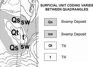
A wide variety of coding conventions had been used to describe similar units in different quadrangles. An effort was made to standardize the codes based on mappers’ descriptions. New codes that were developed as a result of this exercise will be used in future mapping projects (Figures 4 and 5). Undoubtedly because of geologic setting, nonconforming units will be encountered during future mapping projects. In these instances, new codes will be adopted and added to the geologic database.
 |
 |
|
| Figure 4. Surficial unit codes used for 7 different quadrangles. Each column represents a different 7.5 minute quadrangle, while each row represents a different type of surficial unit. The original surficial unit codes varied from quadrangle to quadrangle, but have been standardized using the codes below the table (for example, all codes along the bottom row have been converted to standard code “Qpc”). The codes originally used to describe the surficial unit in row 6 were changed to Qmwd throughout the seven quadrangle area. | Figure 5. Example of surficial unit coding discrepancy. |
Texture codes also were standardized. Figure 6 contains texture descriptions provided by mappers. The descriptions were consolidated into more broadly described texture classes and coded accordingly. However, the original descriptions were maintained in the attribute table in order to preserve the detail recorded by the mapper.
 |
 |
|
| Figure 6. Examples of texture descriptions provided by surficial mappers. Descriptions were generalized into the terms below each box. However, the original, more detailed description used by the mapper also is maintained in the database. | Figure 7. Relatively minor surficial unit discrepancy along quadrangle boundary. |
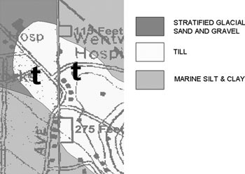
Matters are further complicated by differing interpretations of geologic setting and depositional environment. Although differing opinions are among the driving forces of science, lack of consensus can be very problematic from the cartographer’s perspective. This problem is clearly exposed along quadrangle boundaries where one mappers’ work adjoins another. Many mis-matches in unit boundaries, such as the example in Figure 7, can easily be resolved. Considering the scale at which the geology is mapped (1:24,000), it usually is appropriate to split the difference between polygons. However, some discrepancies in interpretation are often difficult to resolve and usually require additional field work, such as the example in Figure 8.
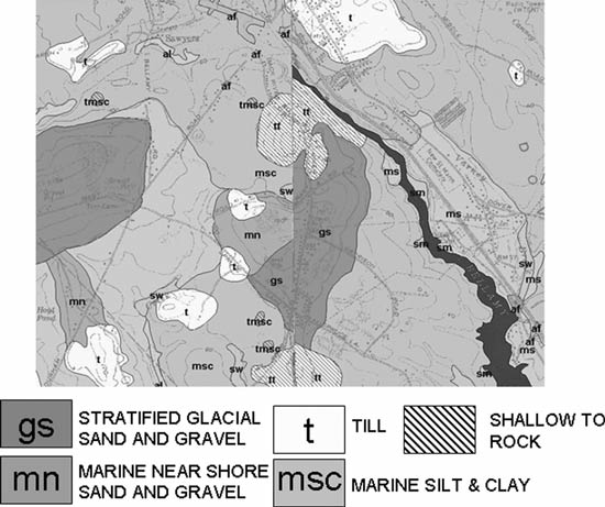 |
Figure 8. Example of surficial unit discrepancy along quadrangle boundary which requires additional field work. |
As noted above, New Hampshire has also adopted a texture region subclass describing the surficial units where appropriate. By utilizing region subclasses, textures may be associated with the surficial units. Region subclasses also help to ensure that texture and surficial unit boundary arcs are edited simultaneously. As with the surficial unit boundaries, textures also need to be edgematched across quadrangle neatlines as illustrated in Figure 9.
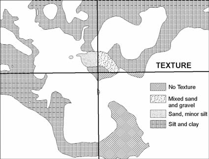 |
Figure 9. Illustration of four adjoining quads that have different polygon textures needing to be resolved. White areas represent surficial units that do not have texture values while polygons with the “no texture” should have a texture and need to be reconciled with their neighboring quadrangle. |
DESKTOP WELL INVENTORY
A desktop procedure for rapidly georeferencing wells has been used to generate data that assist with the resolution of mapping errors. Figure 10 shows georeferenced well data; these give relatively accurate information on overburden thickness and gross material textures, which may provide insight in areas where discrepancies between maps exist.
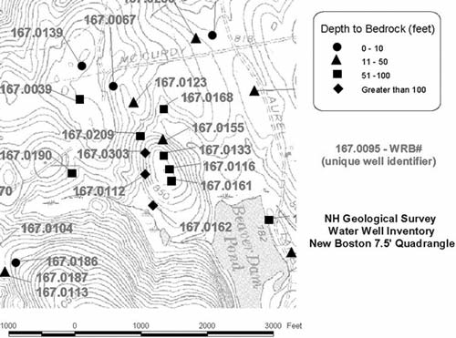 |
Figure 10. Well locations coded by depth to bedrock ranges. The depths are provided by drillers, on well completion reports. The seven digit WRB# (Water Resources Board Number) is a unique identifier assigned by NHGS when the well completion report information is entered into a database. This unique identifier is used to link the georeferenced well location with well construction details in the well database. |
Since 1984, water well contractors have been required by statute to submit a well completion report for any new water well constructed in the state. From that time, the focus has been on digital data storage/retrieval and georeferencing to enable the data to be used in a geographic information system (GIS) environment. However, the labor-intensive effort to field-locate each reported well, initially with traditional map and compass techniques and later with global positioning satellite (GPS) technology, has failed to keep pace with the rate of new well construction. As a result, only 31% of the 93,000+ reported wells have geographic coordinate values.
A decline in staff resources available to georeference the growing backlog of reported wells, combined with a growing demand for georeferenced well data, have provided impetus for developing an alternative approach to locating these wells. Since 1999, the NHGS has been working to develop, test, and refine a desktop GIS well inventory procedure utilizing digital tax maps and digital orthophotography. The procedure is currently being used in a “production mode” to georeference wells in the Seacoast region of the state in order to provide basic data on hydrogeologic conditions.
Tax map and parcel information is obtained from local government officials and is matched to well completion reports. A GIS coverage of map and parcel boundaries is draped over digital orthophotography, and well locations are plotted on housetops with the assumption that the well is in fairly close proximity to the residence (Figure 11).
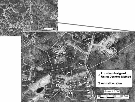 |
Figure 11. Comparison of actual well location and desktop well inventory procedure for georeferencing well locations. The procedure utilizes town map and parcel boundaries draped over orthophotography. |
Location data obtained via the desktop method usually are quite accurate as shown in the chart in Figure 12. In this case, 28% of the wells located do not meet the desired accuracy of 100 feet. However, this population shrinks to only 6% when a 250 foot error is deemed acceptable (Chormann, 2001). Errors are reduced even further if the method is selectively applied to domestic wells and smaller parcels.
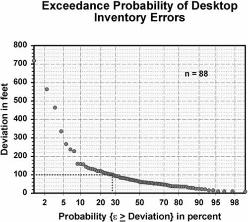 |
Figure 12. Exceedence probability of desktop inventory errors. The y-axis is the deviation (in feet) between the location assigned using the desktop method and the actual location of the well (see Figure 11). The x-axis is the probability (in percent) that a given deviation will be exceeded. |
Over the course of only a few months, NHGS has successfully identified over 1000 well locations to assist with the Seacoast groundwater availability project and the digitization of surficial geologic maps (Figure 13).
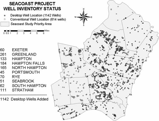 |
Figure 13. Georeferenced well locations added to the Seacoast project area utilizing the desktop inventory procedure. |
CONCLUSIONS
The conversion of paper maps to digital format is a labor intensive process requiring close scrutiny of the maps to be digitized. Identification and documentation of ALL existing features and coding conventions is necessary if standardization is to be applied to the digital data. However, we also must preserve original map content. The integrity of a map may be lost if a feature is changed simply to conform with a standard. Therefore, it is critical to document changes where they occur and to maintain original data within the new map’s database.
Converting maps to digital form creates a much more usable and dynamic product, as the data may be used in conjunction with a wide variety of other datasets. Geologic maps are often a work in progress and by maintaining a product digitally the burden of editing is eased considerably as more information becomes available at a specific location. For example, private lands once closed to entrance may open allowing a geologist to perform field investigations where accessibility was once a problem. New wells may be drilled that provide insight into an area where data was not readily available at the time of map publication. Digital products also provide an easy way of tracking changes to maps so comparisons can be made over time.
Looking into the future, it is important to employ standards in new mapping. With standards in place, mappers may reference specific criteria such as unit coding and descriptions during data collection. By utilizing these criteria before map production, a great deal of time and energy may be saved as new maps can easily and quickly be converted to digital form. Promoting the use of standards will help to ensure that geology is seamless across mapping boundaries and mappers alike.
REFERENCES
Brooks, John, 2004, Surficial Geologic Map of the Northwood Quadrangle, Rockingham and Strafford Counties, New Hampshire: New Hampshire Geological Survey, Geo–166, scale 1:24,000.
Chormann, F.H., 2001, The New Hampshire Water Well Inventory (abstract): 53rd Annual National Ground Water Association Convention and Exposition, Nashville, TN, December 7–9, 2001.
Delcore, Manrico and Koteff, Carl, 1989, Surficial Geologic Map of the Newmarket Quadrangle, Rockingham and Strafford Counties, New Hampshire: U.S. Geological Survey Open-file Report 89–105, scale 1:24,000.
Goldsmith, Richard, 2001, Surficial Geologic Map of the Exeter Quadrangle, Rockingham County, New Hampshire: New Hampshire Geological Survey, Geo–126, scale 1:24,000.
Goldsmith, Richard, 1998, Surficial Geologic Map of the Gossville Quadrangle, Belknap and Strafford Counties, New Hampshire: New Hampshire Geological Survey, Geo–169, scale 1:24,000.
Goldsmith, Richard, 1997, Surficial Geologic Map of the Mt. Pawtuckaway Quadrangle, Rockingham County New Hampshire, U.S. Geological Survey, Open File Map OF97-1,scale 1:24,000.
Goldsmith, Richard, 1995, Surficial Geologic Map of the Alton quadrangle, Belknap and Strafford Counties, New Hampshire: New Hampshire Geological Survey, NH 95–1, scale 1:24,000.
Goldsmith, Richard, 1994, Surficial Geologic Map of the Farmington Quadrangle, Carroll and Strafford Counties, New Hampshire: New Hampshire Geological Survey, Geo–112, scale 1:24,000.
Goldsmith, Richard, 1993, Surficial Geologic Map of the Baxter Lake Quadrangle, Strafford County, New Hampshire: New Hampshire Geological Survey, NH93–01, scale 1:24,000.
Goldsmith, Richard, 1990a, Surficial Geologic Map of the Barrington Quadrangle, Rockingham and Strafford Counties, New Hampshire: New Hampshire Geological Survey, NH 90–02, scale 1:24,000.
Goldsmith, Richard, 1990b, Surficial Geologic Map of the Epping Quadrangle, Strafford and Rockingham Counties, New Hampshire: New Hampshire Geological Survey, NH 90–01, scale 1:24,000.
Gephart, G.D., 1987, Surficial Geologic Map of the Sandown Quadrangle, Rockingham County, New Hampshire: New Hampshire Geological Survey, GEO–91, scale 1:24,000
Gephart, G.D., 1985a, Surficial Geologic Map of the Candia Quadrangle, Rockingham County, New Hampshire: New Hampshire Geological Survey, GEO–90, scale 1:24,000.
Gephart, G.D., 1985b, Surficial Geologic Map of the Derry Quadrangle, Rockingham County, New Hampshire: New Hampshire Geological Survey, GEO–89, scale 1:24,000.
Koteff, Carl, 2004, Surficial Geologic Map of the Parker Mountain Quadrangle, Belknap, Strafford, Rockingham, and Merrimack Counties, New Hampshire: New Hampshire Geological Survey, Geo–139, scale 1:24,000.
Koteff, Carl, 1991, Surficial geologic Map of parts of the Rochester and Somersworth Quadrangles, Strafford County, New Hampshire: U.S. Geological Survey, Map I–2265, scale 1:24,000.
Koteff, Carl, Gephart, G.D., and Schaefer, J.P., 1989a, Surficial Geologic Map of the Hampton and Newburyport East 7.5 Minute Quadrangles, New Hampshire and Massachusetts: U.S. Geological Survey, Open-file Report 89–430, scale1:24,000.
Koteff, Carl, Goldsmith, Richard and Gephart, G.D., 1989b, Surficial Geologic Map of the Dover West quadrangle, Strafford County, New Hampshire: U.S. Geological Survey, Open-file Report 89–166, scale 1:24,000.
Koteff, Carl, and Moore, R.B., 1994, Surficial Geologic Map of the Kingston Quadrangle, Rockingham County New Hampshire: U.S. Geological Survey Geologic Quadrangle Map GQ–1740, scale 1:24,000.
Larson, G.J., and Goldsmith, Richard, 1989, Surficial Geologic Map of the Dover East Quadrangle, New Hampshire: U.S. Geological Survey, Open-file Report 89–97, scale 1:24,000.
Larson, G.J., 1992, Surficial Geologic Map of the Portsmouth and Kittery Quadrangles, Rockingham County, New Hampshire: New Hampshire Geological Survey, Map SG–6, scale 1:24,000.
Sundquist, Daniel, 2000, New Hampshire Towns—Diversity of Density: Society for the Protection of New Hampshire Forests, Concord, NH.