Digital Mapping Techniques '04— Workshop Proceedings
U.S. Geological Survey Open-File Report 2004–1451

Digital Cartographic Production Techniques Using Airborne Interferometric Synthetic Aperture Radar (IFSAR): North Slope, Alaska

By Christopher P. Garrity

INTRODUCTION

In 2003, the Bureau of Land Management, in cooperation with various agencies including the U.S. Geological Survey (USGS), began preparing an Environmental Impact Statement in preparation for potential oil and gas development in the northeastern portion of the National Petroleum Reserve–Alaska. To aid decision-makers in assessing the placement and design of permanent facilities, the USGS was assigned the task of digitizing a series of engineering geologic maps originally published in 1979. Resultant digital maps were incorporated into a Geographic Information System (GIS) project designed to facilitate analysis among federal and industry project managers. A secondary study was to determine the feasibility of using remotely-sensed data to map surficial geology in areas where existing geologic maps were not available. Sensors implemented in the study included Interferometric Synthetic Aperture Radar (IFSAR; http://www.intermap.com/), Landsat-7 Enhanced Thematic Mapper Plus, and Advanced Spaceborne Thermal Emission Reflection Radiometer. This paper focuses on various cartographic production techniques related to data collected by the IFSAR system.

DATA DESCRIPTION

IFSAR data were collected by the STAR-3i airborne synthetic aperture radar system. STAR-3i is a high-resolution, single-pass, across-track IFSAR system, which uses two apertures to image the surface. The path length difference between the apertures for each image point, along with the known aperture distance, is used to determine the topographic height of the terrain. The IFSAR system is capable of collecting data with a vertical accuracy of <1 m and a horizontal accuracy of <3 m.

Data are delivered as three core products: orthorectified radar images (ORRIs), digital surface models (DSMs), and digital terrain models (DTMs). ORRIs are 8-bit grayscale GeoTIFF images that show the radar reflectance intensity of various earth surface materials (Figure 1). These images are commonly used to identify and extract drainage networks and cultural features such as pipelines, roads, and buildings. The ORRIs used in this study had a pixel size of 1.25 m and a horizontal accuracy of 2.5 m. The DSMs, or “first-return” elevation data, display the first surface on the ground that the radar strikes (Figure 2). These images consist of all measured points collected by the sensor, including the z-values of structures (e.g., building and towers) and vegetation (e.g., trees and crops). These elements are removed from the DSM through filtering techniques to create a DTM (Figure 2). The DTMs, or “bald-earth” elevation data, are similar to Digital Elevation Models (DEMs) in that non-terrain elements are absent. However, unlike the regular array of elevation values that are characteristic of a DEM, a DTM defines topographic elements by irregularly spaced breaklines, or abrupt changes in surface smoothness, such as shorelines, roads, streams, and slope breaks. The result is a more accurate depiction of the terrain, which is useful for contouring, TIN calculations, and other terrain modeling.

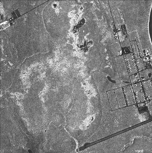Figure 1. ORRI of Nuiqsut area, North Slope, Alaska. Although ORRIs resemble grayscale aerial photographs, each pixel value actually represents the magnitude of sensor signal return.

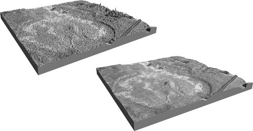Figure 2. Three-dimensional block diagram comparison of DSM (top) and DTM (right), draped with ORRI data, Nuiqsut, Alaska. The DSMs display all of the measured points collected by the sensor, as illustrated by the irregular elevation spikes in the diagram. Non-terrain elements are removed through filtering to create a DTM. The DTMs simulate a “bald-earth” and are traditionally preferred over DSMs for topographic mapping purposes.

STUDY AREA

The study area is located in the Alaskan North Slope along the western edge of the Colville River delta. Bounded by the Beaufort Sea to the north, the study area encompasses nearly 825,000 acres, 95% of which lies in NPRA. The area is completely within the Arctic Coastal Plain, a terrain characterized by a flat to gently rolling tundra-covered surface (Carter, 1985). Toward the coast, the terrain is dominated by periglacial features, including thousands of northeast-trending thaw-lakes. These thaw-lakes are created when ponding of water occurs at the surface, as a result of melting of ground ice followed by surface subsidence. The distinctive elongated shape of the lakes is caused by wave and channel erosion from prevailing winds (Carter, 1985). Inland, the thaw lakes are replaced by meandering streams and treeless areas of tundra vegetation. Elevation in the study area gradually increases in a southerly direction from about 1 to 7 m near the coast, to a maximum of about 50 m at an inland area of large stabilized dunes.

SHADED RELIEF PRODUCTION

Computer-based analytical hillshading has become a widely used tool to visualize three-dimensional topography on a two-dimensional surface. The use of aesthetically pleasing shaded relief images that realistically show topography continues to increase as the quality of rendering software and elevation data improve. Still, it is difficult, if not impossible through purely automated methods to achieve the overall quality of a well-drafted shaded relief map. Unlike manually-produced shaded relief maps, analytical hillshade images often reveal unsightly imperfections in the elevation data used to render the image. The IFSAR data was no exception, and contained flaws in some areas because excess motion in the aircraft caused visible ripples in the dataset. A regular banding pattern was apparent along sensor swath boundaries when elevation data were viewed at small-scales. This aside, the DSMs and DTMs derived from the IFSAR system proved to be an excellent data source for generating shaded relief images.

Large-scale (1:20,000) shaded relief images were generated from DTM data to identify the location of surficial materials with greater accuracy. Initial image rendering revealed potential challenges related to the portrayal of surface features in an area devoid of any significant relief. When rendered with no vertical exaggeration, the shaded relief image resembled a flat, gray rectangle. When a modest amount of vertical exaggeration (5–10×) was applied to the image, shadows appeared blocky and generally were unsightly at the desired map scale. As described below, two graphical techniques (bump mapping and shade softening) were applied to alleviate these aesthetic concerns and to give the landscape images a more natural appearance.

Bump Mapping

Bump mapping is a technique that simulates surface texture through shading. The technique essentially adds detail to a surface without modifying the surface itself, and is widely used in both graphic design and computer gaming. Bump mapping uses a “height map” to simulate surface texture. A height map, which is analogous to a DEM, is a grayscale image that dictates the amount of vertical displacement, relative to adjacent cells, observed in the rendered bump map. Lighter grayscale pixels create a sense of maximum relief, whereas darker pixels have the opposite effect (Figure 3). Bump mapping is especially useful when rendering small-scale to medium-scale 3-D scenes with low resolution DEM data (Figure 4).

Figure 3. The original surface (left), when combined with a height map (middle), results in bump map surface (right). Bump maps are similar to DEMs in that lighter grayscale pixels create a sense of maximum relief, whereas the darker pixels have less of an effect.

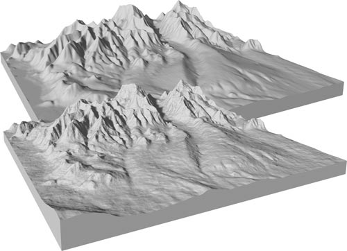Figure 4. Surface model comparison of the foothills area, rendered with 60 m DEM data, Brooks Range, Alaska. The original model (background) was slightly textured by bump mapping (foreground). Bump mapping gives the impression of a more detailed surface through subtle shading.

For the project, DTM surfaces were slightly bump-mapped to generate a hillshade image with a more natural appearance. Because the images were used for surface delineation, a random height map was unsuitable for fear of compromising data integrity. Instead, the corresponding DSM was used as a height map to generate the bumped surface. The natural “roughness” of the DSM gave the hillshaded DTM a subtle texture without obscuring the DTM surface with unnecessary detail. Similar results were achieved in Adobe Photoshop by multiplying DTM and DSM hillshade images with varying vertical exaggerations and layer opacities. However, the bump mapping method proved less time-consuming and provided greater functionality for texture manipulation.

Shade Softening

Shade softening is a technique used to alleviate jagged shades that sometimes appear in automated hillshade images, particularly when vertically exaggerated at large scales. The technique is similar in principle to shadow softening, a computer graphic technique that is applied to 3D objects, rendering object shadows with both an umbra and penumbra(s). In both cases, these softening techniques give the final image or scene a more realistic appearance (Figure 5).

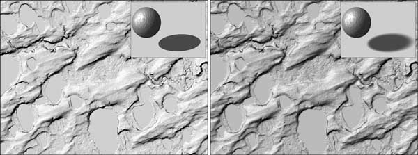Figure 5. Hillshade images rendered without shade softening (left) and with shade softening (right). The shade softening technique smooths blocky shading that is sometimes visible in large-scale automated hillshade images. The technique is similar in principle to 3-dimensional object shadow softening, where shadows are rendered with penumbra effects (right inset), giving them a more realistic appearance than hard shadows (left inset).

For the North Slope project, shade softening was accomplished by generalizing the raw data grid (which smooths, or softens, the irregularities), isolating the shaded pixels, and then merging the softened shade layer with the original grid. To generalize the raw data grid, softening techniques were applied in ArcInfo Workstation by means of various focal functions. The amount of softening was regulated by adjusting the neighborhood configuration (shape, size) in the focal command. In all instances, a very small neighborhood was used and care was taken to not over-generalize the softened grids. The softened grids then were hillshaded in ArcInfo, and were converted to images for editing. By using the “Curves” command in Photoshop, the darkest shades of the softened images were isolated, and all other pixels were converted to white. The adjusted softened hillshade and original hillshade were merged by multiplying the two images in Photoshop with the “multiply” feature in the layers palette. By multiplying the images, the converted white pixels of the softened image were dropped out, resulting in a softening effect restricted to only the darkest shades of the merged image. The resulting hillshade image had a more natural appearance, devoid of any jagged shading.

3-DIMENSIONAL VISUALIZATIONS

3-dimensional visualizations using DTM and ORRI data were generated within the study area to create realistic perspective images and animated fly-throughs. A variety of visualization software packages were used, including Visual Nature Studio (VNS; http://www.3dnature.com/index.html), ArcGIS 3D-Analyst (http://www.esri.com/), Bryce (http://bryce.daz3d.com/), and Terragen (http://www.planetside.co.uk/terragen/). Although each application has unique capabilities, the majority of the visualizations were rendered using VNS. It combines powerful 3-dimensional scene-rendering abilities with traditional GIS functionality, allowing users to import a variety of geospatial data and to work in projected coordinate space. VNS fractalizes terrain objects, giving them more apparent detail by increasing fractal depth. This technique is useful when rendering realistic scenes at large scales, especially in conjunction with bump mapped textures.

The ORRI image data were draped over DTM elevation data in scene-renderings and fly-throughs. The ORRIs were desirable for texture mapping because of their high resolution (2.5m) pixel dimensions. The only limitation was their inherent grayscale color model. To overcome this limitation, the ORRIs were colorized in Photoshop using the “Magic Wand” tool. Grayscale pixels with similar values were isolated and colorized based on the surficial features that they represented. A palette for groundcover colors, derived from colors on digital field photos, was used when colorizing the images. This colorizing method proved to be an inexpensive alternative to purchasing high-resolution color imagery, and the method mimicked true landscape images surprisingly well.

ANAGLYPHS

Grayscale and value-added red-blue anaglyph stereo pairs were created to enhance visualizing and analyzing IFSAR surface data. The anaglyphs were generated using ORRI imagery in conjunction with DTM data to create two slightly differing perspectives of a single image or scene; with one perspective intended for the left eye and the other for the right eye. Upon processing, each ORRI pixel was shifted in the red band depending on the underlying elevation value of the DTM. The processed output was a RGB multi-band image with a shifted red band and identical non-shifted green and blue bands. The processed color image appears gray with purple overtones to the naked eye when a grayscale ORRI is used. When viewed through red-blue glasses, the same image displays a vertically-exaggerated surface (user defined) in three dimensions.

Value-added color anaglyphs (Figure 6) were more difficult to produce due to limitations in color choices when colorizing the ORRIs. Colors with high red, blue, or green content were not complementary to anaglyph processing, and they tended to interfere with the three dimensional visualization effect. In addition, the anaglyph glasses themselves revealed false-colors due to the red-blue film, further limiting desirable color choices. Adjusting the intensity of the anaglyph red channel in Photoshop minimized the color interference, but did not eliminate the interference problem altogether.

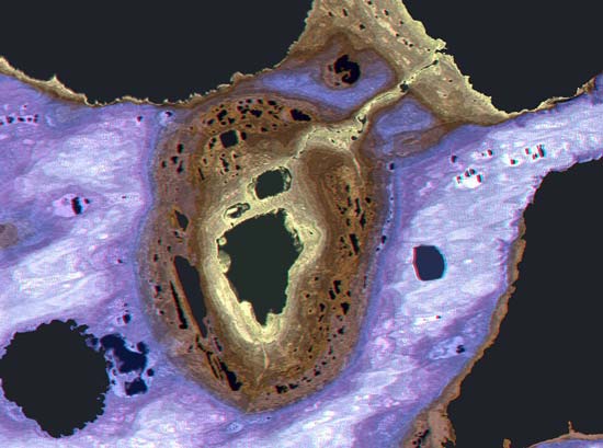Figure 6. Color anaglyph of some of the numerous thaw lakes in the North Slope of Alaska. When viewed through red-blue glasses, the topography is seen in three-dimensions (online version only). The ORRI was value-added with an elevation color ramp, and the underlying DTM was exaggerated to accentuate surface features. This figure is represented here in black & white, but is available in color in the online version of this publication.

REFERENCES

Carter, L.D., and Galloway, J.P., 2005, Engineering geologic maps of northern Alaska, Harrison Bay quadrangle, with a section on The digitally revised engineering geologic maps of northern Alaska by D.W. Houseknecht, C.P. Garrity, and D.C. Meares: U.S. Geological Survey Open-File Report 2005-1194, available only online at http://pubs.usgs.gov/of/2005/1194/. [Supersedes Open-File Report 85-256.]