Digital Mapping Techniques '04— Workshop Proceedings
U.S. Geological Survey Open-File Report 2004–1451

Creating 3D Models of Lithologic/Soil Zones Using 3D Grids

By Skip Pack

THE PROBLEM AND THE GOAL

Aside from describing and recording surficial geology, mapping of the subsurface is, for geologists, one of the most frequently performed tasks. Traditionally, surface contacts are integrated with data gathered in vertical borings, usually drillers’ logs, and correlations are manually interpreted on sections between the borings. Contour maps can then be made, manually, or by computer from the surface and correlated borehole data. In this paper, I will describe a work path using the same data, but bypassing the manual correlation step, to create a 3D model of zones (volumes) representing soil or lithology categories or types, or even larger scale geologic zonation. Maps of zone tops, if needed, can then be calculated from the 3D model with rigorous interzone consistency. This involves a pastiche of known techniques, and offers real advantages in some cases, and none in others.

The process using traditional manual correlation works very well when each zone can effectively be defined with a top and bottom surface, that is to say there is little or no lobing or interfingering of zones, and when zones extend far enough to be encountered in several borings. If the geologic environment is relatively chaotic over short distances relative to the spacing of borings, traditional correlation becomes difficult or impossible. Glacial and fluvial environments commonly produce deposits that are difficult to correlate over even short distances.

In our method, we begin by creating an indicator variable for each possible soil or lithology type at each data location, whose value simply indicates whether each type of material is present or absent. Using those indicators as input to 3D grid calculation results in a grid which estimates the likelihood of occurrence of each soil/lithology type at each node of a 3D grid. Because each grid was calculated independently from those representing other soil/lithology types, there will be locations away from the sample points where more than one type is shown to probably exist. This requires a reconciliation process, which I will describe, that determines which soil/lithology type is most likely at each location. Finally, I will describe a method for labeling each separate occurrence of a given type, rather than grouping them. For example, we can create a number of zones, each representing a distinct, separate sand lens, rather than lumping them all together as a single discontinuous sand zone.

Several organizations have found this method useful when manual correlation is difficult or impossible to achieve. I also believe that this method may prove useful as a precursor to manual correlation. Once a model has been created using this method, model-derived cross sections can be generated on traverses using the boring locations as vertices. Use of these cross sections as background reference for the manual correlations may offer time savings over the purely manual process. The geologist starting with the model-derived sections would need only to focus on correcting the geologically implausible aspects of the automated method output.

I have used EarthVision (EV), a geologic modeling software package from Dynamic Graphics, Inc., my employer, to implement this process. I will, in this discussion, focus on the conceptual process, which could be implemented using tools and software packages from other sources.

A SIMPLE TEST CASE

This technique requires a data set of lines, each having numerous points, where each point indicates the local soil or lithology (i.e., each line is a continuous, vertical sampling through the soil, sediment, and/or rock in the study area). Vertical borings are the most common source of such data, and can be conventional wells, test borings, or data gathered by direct push technologies such as cone penetrometers. In many cases, the data points are derived by interpolation or expansion of the actual information available for the borehole. For example, a driller’s log indicating the top of each zone implicitly states that more or less the same material exists until a change is logged that indicates a new material. A script or spreadsheet would then be used to fill in the intervening interval with the value from the last log entry uphole. The following is an excerpt from a cone penetrometer data set. The first three columns contain the X, Y, and Z coordinates of the data point and the fourth column contains an integer code for the soil or lithology type encountered. The header line that begins with # Description matches the integers 1, 2, and 3 with the soil category names. The Z field (or column) of data is expressed in units increasing upwards both above and below a 0 datum, which, in this case, is mean sea level. Figure 1 provides a perspective view of this data.

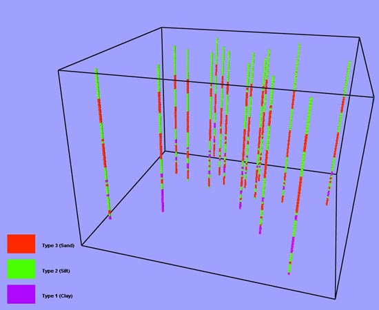Figure 1. Input data file indicating soil types interpreted from cone penetrometer tip pressure and sleeve friction readings processed through a lookup table to determine soil/lithology type. Since cone penetrometer readings are almost continuously sampled, the data points (small cubes) in the illustration are measured points.

# Type: property scattered data
# Version: 7
# Description: 1=clay, 2=silt, 3=sand (soilcat)
# Format: free
# Field: 1 x
# Field: 2 y
# Field: 3 z
# Field: 4 soilcat
# Projection: Local Rectangular
# Units: unknown
# End:
14191624.16 1270905.512 -7.42 1
14191624.16 1270905.512 -6.77 1
14191624.16 1270905.512 -0.86 1 14191624.16 1270905.512 1.11 1
14191641.82 1270917.503 -6.11 1
.
.
.
14191624.16 1270905.512 -8.73 2
14191624.16 1270905.512 -8.08 2
14191624.16 1270905.512 -6.11 2
.
.
.
14191624.16 1270905.512 -9.39 3
14191624.16 1270905.512 -4.8 3
14191624.16 1270905.512 -4.14 3

The next step is to create one new column per soil/lithology type. In this case, there are three types, so we create an indicator value for each type and record it in the type-specific column. Using a spreadsheet, a script, or a suitable program, we tested the integer value in the fourth column of the original file and set the appropriate indicator column to “1” where that type occurred at that location and “0” where it did not. The following is an excerpt of that file after the indicators were added:

# Type: property scattered data
# Version: 7
# Description: Created with formula processor (skip, 30 Mar 2003)
# Format: free
# Field: 1 x
# Field: 2 y
# Field: 3 z
# Field: 4 soilcat
# Field: 5 I_one
# Field: 6 I_two
# Field: 7 I_three
# Projection: Local Rectangular
# Units: unknown
# End:
14191624.16 1270905.512 -7.42 1 1 0 0
14191624.16 1270905.512 -6.77 1 1 0 0
14191624.16 1270905.512 -0.86 1 1 0 0
.
.
.
14191624.16 1270905.512 -8.73 2 0 1 0
14191624.16 1270905.512 -8.08 2 0 1 0
14191624.16 1270905.512 -6.11 2 0 1 0
.
.
.
14191624.16 1270905.512 -9.39 3 0 0 1
14191624.16 1270905.512 -4.8 3 0 0 1
14191624.16 1270905.512 -4.14 3 0 0 1

Using this augmented file, I calculate one 3D grid per category using the indicator data for that category as input. With most “representational” or deterministic gridding methods (which models natural surfaces or volumes as opposed to analytical gridding like trend surface analysis), the resulting grid node values will have values from around 0.0 to around 1.0; but, unlike the input values (0.0 or 1.0), they will vary continuously where the grid nodes are interpolated or extrapolated. This transformation from the discrete input values to the continuously varying grid node values creates a probability-like value that expresses the likelihood of the soil/lithology type existing at each node location.

If you choose kriging for this gridding step, you are following a very standard path that has long been used on discrete data. This is not to be confused with indicator kriging using thresholds on continuous data. In this case I used EarthVision’s 3D minimum tension gridding, though I have also used simple nearest neighbor gridding, where the gridder sets each node to the value of the nearest input data point. Initial tests suggest that the results are a little less sensitive to differences in gridding techniques than single grids calculated from continuous numeric input variables, but not enough cases have been run to state that with any conviction. Kriging would be desirable when variogram analysis or prior knowledge of the area indicates anisotropic variation in the zonal orientation. Without some indication or prior knowledge regarding the existence and nature of the anisotropy, deterministic gridding methods will yield a defensible result more quickly, and, potentially, with fewer gridding artifacts.

The resulting grid, using a higher order gridder like a minimum tension algorithm, will have node values ranging from somewhat below 0 to somewhat above 1. A linear weighted average gridding algorithm likely would have values ranging from slightly above 0 to slightly below 1, unless a node happens to be coincident with a data point. In that case, 0 or 1 would be assigned to the node. In any case, the resulting grid contains values that I would call pseudo-probabilities. While I am not sure that there is any statistical rigor in their generation, they serve well when used as probabilities. When the values exceed 1 or fall below 0, their qualification as probabilities is dubious by definition, but this seems not to matter in practical terms since the comparison of the “probabilities” of several soil/lithology types at any one node is only in question when two or more types have similar “probabilities”. In this case, the “probabilities are likely to be well inside the 0-to-1 range. Thus, where a soi/lithology type shows a value greater than 0.5, it is assumed to exist at that location. Figures 2 and 3 show the volume for the Type 1 (Clay) grid above 0.5 represented by blocky cells and by smooth contour surfaces. These are two representations of the same grid, with the difference in display resulting from 3D viewer options.

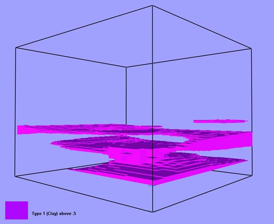Figure 2. Type 1 (Clay) 3D grid where pseudo-probability is > 0.5 (cells shown as voxels).

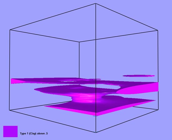Figure 3. Type 1 (Clay) 3D grid where pseudo-probability is > 0.5 (3D oblique contouring).

Reconciliation

Because these grids of individual soil/lithology type probabilities are created independently, the sum of the probabilities at each grid node location does not equal 1.0, except for those locations where a sample point is coincident with a grid node. For this reason, it is almost certain that there will be node locations where more than one type is indicated to be likely to exist. Thus, the next step is a reconciliation process to select only one type as present at each grid node location.

I have simply compared the grid node values of each of the soil/lithology type grids at each location and selected as present the type with the highest pseudo-probability. I can then create a single 3D grid containing an integer value showing which type is present, in the same way that integers were used in the unmodified input file.

This method of reconciliation has been used on a number of projects to date (approximately 6), and has served well. At most node locations, the choice of which soil or lithology type is present is quite clear, that is to say, the pseudo-probability of one type is distinctly higher that those of the other categories. However, some node locations may have pseudo-probability values for one or more types that have very similar values. At those locations, selecting the highest numerical is somewhat crude and questionable. Use of secondary information derived from geophysics or stochastically inferred tendencies could greatly improve the reconciliation process.

Model Building

I have, so far, generated and used two outputs from the reconciliation process. The first is the combined integer grid described above. The second is a set of individual soil/lithology type grids indicating that the type is present or absent at each grid node. Thus, with three soil/lithology types, we have three reconciled grids containing indicator codes, identical in concept to the indicator codes in the modified input file where the indicators were put into three additional fields. In this case each node of the grid indicates present or absent. Earthvision allows us to create volumes with oblique boundaries that contain the soil/lithology types from 3D grids. These volumes can then contain properties such as porosity or hydraulic conductivity (permeability) that can, in turn, vary continuously in three dimensions within each zone, but discontinuously from zone to zone. Figure 4 shows a reconciled 3D grid of combined zones cut away to display the internal variation. The “blocky” nature of the grid is obvious. Figure 5 shows a model with the clay zone projected into a cutaway. The smoother representation using oblique triangles is based on the same grids shown in Figure 4.

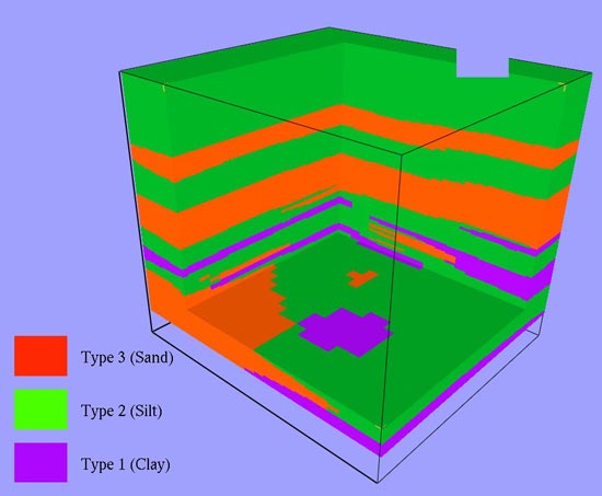Figure 4. Combined, reconciled 3D grid of all soil/lithology types.

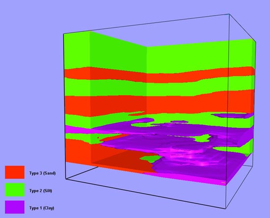Figure 5. 3D volumetric model with clay zone displayed in cutaway.

You will notice the multiple occurrences of the clay zone, which may or may not be connected outside of the model volume. This leads to the next topic, differentiation between potentially separate occurrences of similar or identical soil/lithology types, that is to say, spatially separated volumes where the same type was assigned during the input data interpretation.

Clustering (3D volumetric classification)

A final, and very interesting, step in this technique is processing the combined integer grid to detect and label each volumetrically separate occurrence of each soil/lithology type. Graham Brew, of Dynamic Graphics, has developed a script that uses the 3D grid containing integer soil/lithology codes output from the reconciliation process. The output of this script is also a 3D grid of integer values, but these integers are compound labels that show both the soil/lithology type and a unique integer value for each spatially separate volume where that type is present. These separate volumes are sometimes referred to as “geobodies”.

In essence, this process involves starting at one node location, determining what type is present at that node, then looking at each adjacent node and determining if the same type is present. The script repeats this process, looking vertically and horizontally until all adjacent nodes of the same type have been detected. All of the adjacent nodes are given a unique label and written to the output grid. The script then moves on to the next node in the input grid, which has not yet been labeled, and conducts the adjacency process again to build the next geobody.

In the sample case used here, the 3D grid output from the reconciliation step contained values of 1, 2, or 3 indicating clay, silt and sand, respectively. The output of the clustering script output values of 1 and 2 for each of the two clay bodies, 18, 19, and 20 for each of the three silt bodies, and 44, 45, 46, and 47 for each of the four bodies of sand. These numbers are arbitrary and have no significance beyond designating a separate integer per body while still indicating the soil/lithology type. Using this grid to generate a 3D model with oblique zone boundaries, we can see each of the sand zones projected into the cutaway model in Figures 6, 7, and 8.

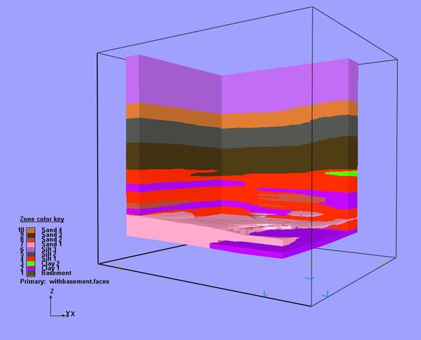Figure 6. Sand Zone 1 projected into cutaway model.

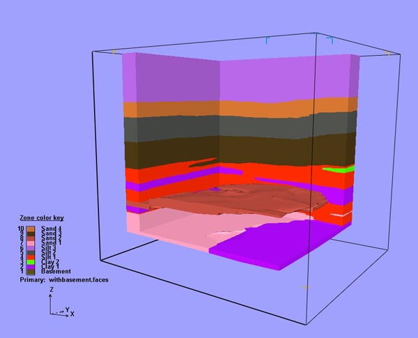Figure 7. Sand Zone 2 projected into cutaway model.

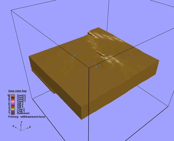Figure 8. Sand Zones 3 and 4 shown in isolation.

There are a number of issues to resolve in the clustering process, which I will not discuss in detail. They are generally simple, and can be addressed in the script used for the process. One example is the degree of spatial adjacency of grid nodes required for assignment to the same geobody. Generally, nodes of an identical soil/lithology type, which are above, below, or directly beside, are considered to be in the same body. It is less simple when the adjacency is diagonal laterally, vertically, or both. The user needs to determine if this diagonal adjacency is sufficient to provide a geobody connection.

Similarly, it is useful to avoid classifying nodes into geobodies where the “zone” created would be too thin or too small in volume. A frequent complication of the clustering/classification process is creation of a “noisy” volume with a large number of small, separate bodies. As always, you must select the resolution (scale or granularity?) of your classification based on the uses to which the result will be applied. The overall goal in visualization or further analysis should determine the level of generalization you select in the clustering process.

One natural result of applying rules for geobody generation, such as those discussed above using adjacency, thickness, and volume, is the generation of some number of unclassified (formerly classified before the clustering) cells. Development of rules that can be used to select the most appropriate adjacent geobody type into which each unclassified cell should be merged is one of the current topics under consideration.

While the clustering process presently used in this larger technique is relatively simple and deterministic, it has worked quite well on several cases. This is a natural area for more sophisticated stochastic methods, which could allow for inclusion of anisotropic/directional continuity determination.

CONCLUSION

This general technique for generating 3D models of zones from data that indicates soil/lithology types has worked well in a number of cases. The data set and model used in this paper cover a very small area in a glacial environment. The largest number of soil/lithology types that we have used in a model with this technique is 24, and the largest range of a model thus far is 42 km × 40 km × 2 km. In the example used in this paper, another model was generated using traditional correlation prior to model generation. The traditionally correlated model had somewhat less detail as a consequence of each zone being modeled with only a top and bottom surface (no intricate lobing). In the wide-area model mentioned above, traditional methods were used to develop a Paleozoic basement surface and a top of Tertiary volcanics surface, with the 3D method described here used for five shallow, mostly unconsolidated, units in between.

Early in this paper I mentioned the potential use of this method as a timesaving precursor to traditional correlation. To date, no one who has used this method has gone back and performed the 3D model supported manual correlation/edit, though I believe this is desirable for quality control. The modest number of projects performed thus far suggest that this 3D automated technique can perhaps reduce time needed to complete the model by about 75 percent compared to traditional methods. In the other two cases mentioned above, the 24-zone case and the wide-area model, traditional methods would have been very difficult or impossible within a reasonable timeframe.

There are many promising avenues for improvement and extension of the workflow outlined above. Both the reconciliation and clustering/classification steps seem to be natural candidates for application of stochastic techniques such as those included in the transitional probability methods developed by Weissmann, Carle, and Fogg (1999). Additional value should be available through use of geophysical data to help differentiate between soil/lithology types when the basic method does not indicate a clear choice. Graham Brew has made improvements to the clustering methods recently, and I have begun to study the reconciliation process to gauge which node locations are candidates for use of secondary data such as gamma ray, resistivity, and statistically inferred criteria.

REFERENCE

Weissmann, G.S., Carle, S. F., and Fogg, G. E., 1999, Three-dimensional hydrofacies modeling based on soil surveys and transition probability geostatistics: Water Resources Research, v. 35, no. 6, p. 1761–1770.