Digital Mapping Techniques '04— Workshop Proceedings
U.S. Geological Survey Open-File Report 2004–1451

Exploring Shaded Relief: The Shaded Drift-Thickness Map of Ohio

By Donovan M. Powers

INTRODUCTION

Shaded relief images have become a popular and useful means for improving the “readability” of geologic maps. Some important considerations when evaluating the possibility of using shaded relief for a given map application are: availability of suitable digital elevation data, extent to which available digital elevation data will need to be corrected/enhanced for the intended application, and how other cartographers and Geographic Information System (GIS) professionals are currently using the dataset. The intended end-uses of the shaded relief could have an effect on the methods and formats you use in deriving the data. GIS professionals may use a variety of different software packages and your final output may need to conform to a standard format in order to accommodate various users. Maintaining communication with other professionals could save you some time and effort, and help you to standardize your products.

Digital elevation data generally is available for any area of the United States at no cost. However, if the available data is not sufficiently detailed for your intended application, you may need to create your own dataset. Sometimes, available data must be heavily edited and corrected in order to be suitable for your intended use. In most instances, conscientious cartographers will want to edit and enhance any publicly available digital elevation dataset before using it on their mapping product. This can be a very detailed and time consuming process, but the final product will give you great satisfaction and provide you with an excellent elevation dataset that can be used for many other map applications. This paper describes some techniques used to create a statewide shaded-relief image (Powers and Swinford, 2004; Figure 1).

GETTING THE DATA

When creating an ArcGrid elevation dataset, you will want to select a dataset or create one with a cell size appropriate for your scale or resolution of mapping. These datasets, or Digital Elevation Models (DEMs), are available from the U.S. Geological Survey (USGS). The most complete coverage is available through their National Elevation Dataset (NED); this dataset has a 30-meter spacing. Higher-resolution data (e.g., 10-meter grid) and lower-resolution data (e.g., 90-meter grid) also are available for selected areas of the U.S. The NED and other DEMs can be obtained from the USGS Earth Resources Observation Systems (EROS) Data Center (USGS EROS Data Center, 47914 252nd Street, Sioux Falls, SD 57198; http://edc.usgs.gov/products/map/dlg.html). NED data is useful for cartography at scales of about 1:100,000, or smaller (e.g., 1:250,000). If your map is a larger scale, then you will need to create or obtain a higher resolution (smaller cell size) dataset. If the higher-resolution DEM’s are not available for your area of interest, you can follow the process outlined by Haugerud and Greenberg (1998) to create your own. This process, presented at the 1998 Digital Mapping Techniques workshop, utilizes ESRI’s ArcInfo Workstation to create an ArcGrid file based on DEM or Digital Line Graph (DLG) layers available through the EROS Data Center.

The Drift Thickness Map of Ohio (Figure 1) was created from the Ohio Division of Geological Survey’s bedrock topography contours and converted to a surface using Haugerud and Greenberg’s methods. This surface was then subtracted from the DEM (earth’s surface) to yield a thickness of drift. From the thickness layer a hillshade layer was created, converted to an image, and cleaned in a graphics program.

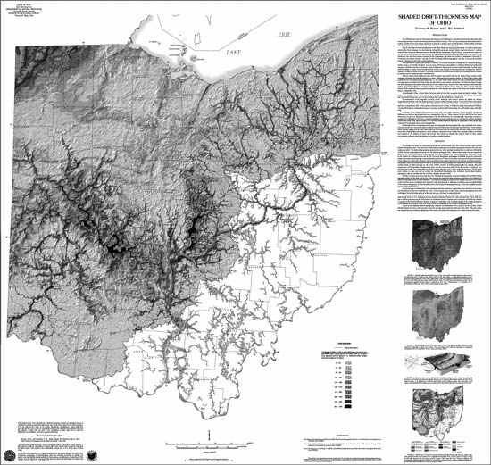Figure 1. The Shaded Drift-Thickness Map of Ohio.

CLEANING THE SHADED RELIEF

Many GIS professionals already have some type of shaded relief data on hand that has not been “cleaned” (i.e., edited and corrected)—probably for lack of time. Nonetheless, a proper cleaning is essential before an elevation dataset is used in a published product.

Upon close inspection of the unclean data, you may notice artifacts or “terracing” (Patterson, 1997) in your shaded relief layer that correlate to the topographic contours from which your DEM was created. A slight bias in the interpolation algorithm that Arc Workstation uses to create surface grids causes input contours to have a stronger effect on the output surface than areas between the contours. This bias can result in a slight “flattening” of the output surface as it crosses the contour. This may result in misleading results when calculating the profile curvature of the output surface. Recently, a new version of the algorithm has been released claiming to address this issue. The algorithm could reduce the amount of time it takes to clean a DEM. It is available as a standalone application with a graphical user interface. The version ESRI uses is substantially older and does not incorporate the additional functionality. It is unknown if or when ESRI will implement this version (Hutchinson, 2000; 2004).

Using tools such as Arc Workstation or Adobe Photoshop, you can accomplish a significant amount of data cleaning without compromising data integrity. In Arc Workstation, the FOCALMEAN command can be used to smooth out unwanted artifacts. FOCALMEAN includes in its calculations a specified cluster of cells (a “neighborhood”) around each cell. You specify the size and shape of the neighborhood, and FOCALMEAN calculates the average of the value of the neighborhood. In many cases, you can use a circle with a 5 or 7 cell radius to smooth the raster, depending on the extent and resolution of your data. This doesn’t always take out all of the artifacts but it will smooth them for a cleaner look. As you get familiar with the commands, you might find other ways to clean your data. Presently, this seems to be the best approach to eliminate a majority of the artifacts, but I am eagerly awaiting a more comprehensive method.

Should you want to further clean the data, you can use a graphics program like Photoshop. By editing the appearance of a hillshade image created by ArcGrid rather than editing the elevation data, you can greatly enhance your final output. Convert your hillshade grid into a gray-scale tiff and edit it in your graphics/photo program using the filters and tools to smooth out the “plateau” or “terracing” effects. This step requires practice and time. Be careful not to overuse the tools. The rubber stamp, dodge, burn, blur, and airbrush tools are the most useful. Some 3rd party add-on filters might also be helpful.

Another option to better display your hillshade is to enhance the peak and valley tones (Figure 2). There is a tendency to lose data on either end of the tonal scale—light values (less than 5 percent) usually disappear completely and dark values (greater than 90 percent) fill in and appear solid. For example, steep slopes perpendicular to the illumination direction appear washed out, whereas shadowed slopes become solid black (Patterson and Hermann, 1997). Blending two separate renderings of the hillshade images can emphasize the subtle details that would likely be lost using the typical software application. Blending uses two copies of the hillshade image overlapping each other. The uppermost copy can be rendered with a lower percentage of transparency, roughly 60% depending on the strength desired, and the histogram, or the contrast can then be adjusted to allow details to appear in the darker and lighter areas. The layers can be merged into one once the desired effects have been achieved.

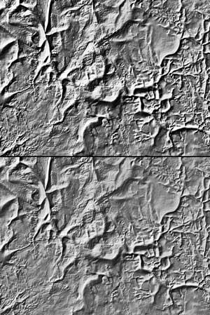Figure 2. A portion of the Shaded Drift-Thickness Map of Ohio, before (top image) and after (bottom image) value-enhancing the tonal qualities to improve the depiction of topographic relief.

USING THE SHADED RELIEF

Cartographers use several methods to create shaded relief images, and the correct choice for you depends on the kind of map you are producing and the software package with which you intend to produce the map. Many cartographers use ESRI products for data creation, and export the data into graphics software such as Adobe Illustrator or Macromedia’s Freehand for production of a final product. The best approach is to work with various programs since no single software package seems to be able to adequately handle all of these steps.

If you are making a geological map and wish to add shaded relief to emphasize topographic features, you will want to make the geology somewhat transparent and place that layer over your hillshade. You could do the opposite and make the geology the topmost layer and give it transparency; I generally place the hillshade as the topmost layer with transparency, for a few reasons. While creating the map, I often turn the hillshade off for faster digital rendering. Having the geology with no transparency allows printing without hillshade for geology editing during early inspections. The use of layers and transparencies can be implemented in nearly all of the software packages you might be using. The percentage of transparency depends on your needs, the software you are using, and how you want your map to look. ESRI’s products use percentages of transparency whereas Adobe’s products use percentages of opacity—a slightly different approach, but the same effect can be accomplished.

If you are making a shaded relief map with elevation intervals shown in different colors, you can do this by either of two methods. The first option is to use two separate layers, one for the colors of the elevations, and another for the hillshade. In this approach, a transparent hillshade layer is draped over a separate layer of color-coded elevation polygons to achieve a textured elevation map. The other option is to merge these two layers together using ArcInfo Workstation, ArcMap, or Photoshop, depending on the format of your data. I prefer to keep the elevation or geology separate from the hillshade in the event the map will be sent out for printing. The colors will be divided into color separates and having the hillshade on its own layer as a separate color will allow you to keep a similar appearance to what you have on-screen during digital compilation. When merged, the shading becomes part of the underlying colors of geology or elevation and the final print colors will not be what you anticipated. Another reason I don’t merge the hillshade is simply to have them available for use in other projects as individual layers. You may find it beneficial to merge the two layers in certain situations. One merged layer would have a smaller file size and use less hardware resources than working with two separate layers would. When you compile a final layout this small detail could be the difference between making a print and crashing your computer while attempting to print. Minimizing the size of your digital file also reduces the processing time.

REFERENCES

Haugerud, R., and Greenberg, H.M., 1998, Recipes for Digital Cartography: Cooking with DEMs, in Soller, D.R., ed., Digital Mapping Techniques ’98—Workshop Proceedings: U.S. Geological Survey Open-File Report 98–487, p. 119–126, accessed at http://pubs.usgs.gov/of/of98-487/haug2.html.

Patterson, T., and Hermann, M., 1997, A Desktop Approach to Shaded Relief Production: North American Cartographic Information Society (NACIS), Cartographic Perspectives, no. 28, p.38.

Patterson, T., 1997, Creating value-enhanced shaded relief in Photoshop: NACIS Cartographic Perspectives, no. 28, accessed at http://www.shadedrelief.com/value/value.html.

Hutchinson, M.F., 2000, Optimising the degree of data smoothing for locally adaptive finite element bivariate smoothing splines: Australian & New Zealand Industrial and Applied Mathematics Journal, v. 42(E), p. C774–C796, accessed at http://anziamj.austms.org.au/V42/CTAC99/Hutc/Hutc.pdf.

Hutchinson, M.F., 2004, The Australian National University, Centre for Resource and Environmental Studies, ANUDEM, accessed at http://cres.anu.edu.au/outputs/anudem.php#3.

U.S. Geological Survey, 1990, Digital Elevation Models: U.S. Geological Survey, Data Users Guide 5, 51 p.

Powers, and Swinford, 2004, Shaded Drift-Thickness Map of Ohio: Ohio Department of Natural Resources, Division of Geological Survey, Map SG-3, 1:500,000 scale, accessed at http://www.dnr.state.oh.us/geosurvey/pdf/sg3map.pdf.