Digital Mapping Techniques '04— Workshop Proceedings
U.S. Geological Survey Open-File Report 2004–1451

Surface Terrain of Indiana—A Digital Elevation Model

By Robin Rupp

INTRODUCTION

The surface terrain dataset of Indiana was created using part of the U.S. National Elevation Dataset (NED) and newly-created digital elevation models (DEMs). New digital elevation data was processed into new DEMs and served to replace 275 of the 710 7.5-minute quadrangles within the Indiana portion of the NED.

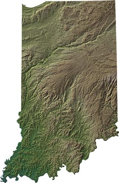
This report describes the processes of 1) creating new DEMs, 2) merging the new data and the NED into a new dataset for Indiana, and 3) creating TIFF images from the final dataset. The revised digital elevation model for Indiana and parts of the surrounding states is available on a CD-ROM (Brown and others, 2004) as raster data in ESRI Grid format. This report also provides the background for the Indiana Geological Survey Poster05 (Berry and others, 2004; Figure 1) and the forthcoming terrain image series.

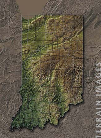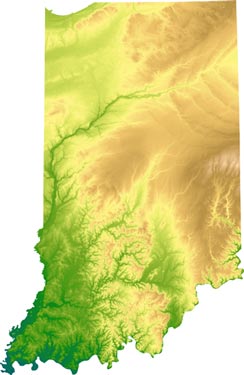
Figure 1. Surface Terrain of Indiana from IGS Poster 5. In this image, the revised digital elevation model has been exported from ESRI ArcView and brought into Adobe Illustrator/Avenza MapPublisher (http://www.avenza.com/main.html) and Adobe Photoshop for enhancement.

NATIONAL ELEVATION DATASET

The National Elevation Dataset (NED) is a relatively new raster product created and maintained by the U.S. Geological Survey (USGS). The data and information about the NED are available at http://gisdata.usgs.net/ned/ and http://mac.usgs.gov/isb/pubs/factsheets/fs14899.html, respectively. It provides seamless elevation data over the entire United States at approximately 30-meter resolution. The USGS envisioned this dataset as a vehicle to allow users to focus on analysis rather than data preparation. They created the NED from a variety of digital elevation model sources that had various horizontal datums, map projections, elevation units, and quality. In 1999, the Indiana Geological Survey (IGS) acquired the NED for Indiana and parts of Illinois, Michigan, Ohio, and Kentucky; at that time, it was the best available DEM of Indiana at 30-meter resolution.

REVISING THE INDIANA DEM

The majority of the NED is high-quality (Level 2) DEM data, however, a part of the data is lower-quality (Level 1) data. Level 1 DEMs were created with older methods and have lower accuracy standards, while Level 2 DEMs were created using more modern methods and have higher accuracy standards (Figure 2). The IGS discarded the Level 1 data in the greater Indiana area of the NED and replaced it with newly created digital elevation models (DEMs). In the process of making these DEMs, it was necessary to reprocess some of the high-quality (Level 2) quadrangles owing to their location within blocks of Level 1 data (Figure 3). Of the 275 7.5-minute quadrangles replaced in the Indiana dataset, 216 quadrangles were Level 1 and 59 quadrangles were Level 2. Other revised areas (shown on Figure 3) are: 1) a part of western Ohio, including the eastern portion of Allen County, Indiana, which was processed by the Ohio Division of Geological Survey; 2) sixteen 7.5 minute quadrangles in and adjacent to Berrien County, Michigan; and 3) a 1000-meter buffer zone, extending just beyond the block of replaced quadrangles, which was added in order to create a more seamless splice at the edge of the newly created quadrangles.

A		B
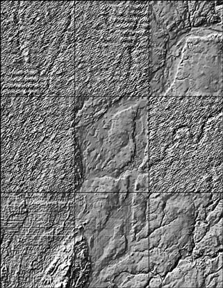
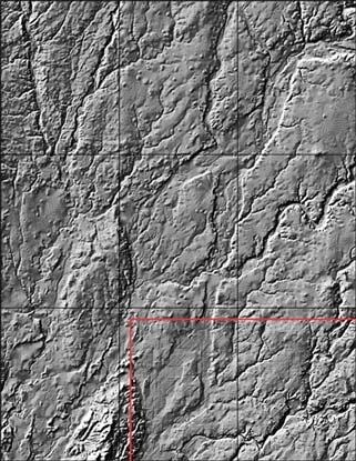
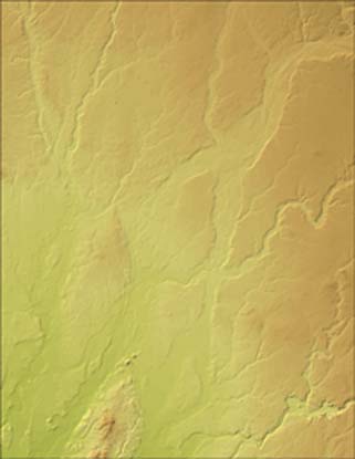
C		Figure 2. The digital elevation model of nine central Indiana 7.5-minute quadrangles before (A) and after (B and C) the editing process. A. Original NED, hillshaded. Five quadrangles are Level 1 (lower-quality) data and four quadrangles are Level 2 (high-quality) data. In the editing process of this area, the IGS replaced all the Level 1 quadrangles and two Level 2 quadrangles (the northeast and central quadrangles) with new digital elevation models made by the IGS. The south-central and southeast quadrangles were outside the revised area. B. Revised DEM, hillshaded. There is a slight difference in topographic “texture” between the areas processed by the IGS and the areas processed by the U.S. Geological Survey (southeast and south-central quadrangles). C. Revised DEM, with a color ramp and the hillshade. This is the same edited DEM as in B., but with color applied according to elevation combined with the hillshade.

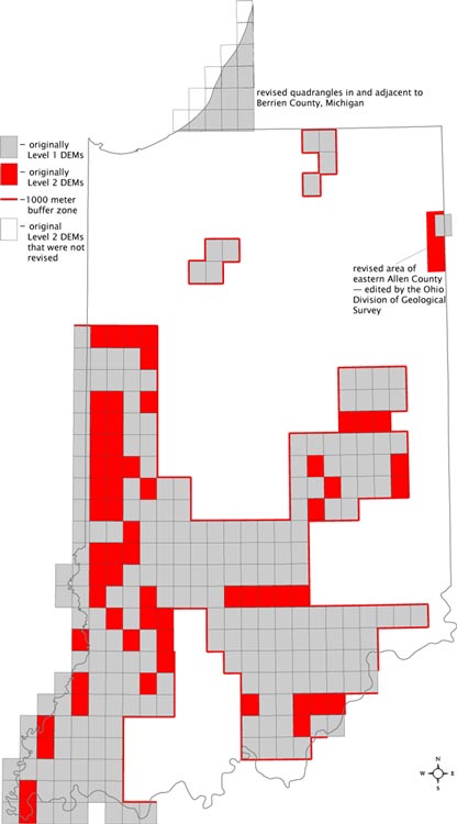Figure 3. Revisions in the DEM dataset of Indiana.

The processing steps to create the DEMs in ArcInfo 8.2 are listed in the Appendix. This processing included the following components:

• digital hypsography—contour data provided the elevation values for the DEM. The USGS completed Indiana hypsography at 1:24,000 scale in 2003.
• digital waterbody boundaries—waterbody polygons are needed to ensure that lakes appear flat in the resulting DEM. These were obtained from the U.S. Census Bureau 2000 TIGER/Line files (1:100,000 scale) and the USGS/EPA National Hydrography Dataset (1:100,000 scale).
• digital hydrography—oriented stream data provide the direction of the slope, and ensure the correct placement of the stream valleys. These data were obtained from both the U.S. Census Bureau 2000 TIGER/Line files (1:100,000 scale) and the USGS/EPA National Hydrography Dataset (1:100,000 scale).

ELEVATION DISCREPANCIES

Despite our processing, elevation discrepancies may exist in the DEMs for some of the reprocessed 7.5-minute quadrangles for the following reasons:

• Some of the digital hypsography contains incorrect elevation data. These were not corrected because there appear to be very few of these errors and the datasets were large.
• The lake polygons and stream paths from the TIGER dataset adhere to a (USGS) 1:100,000 scale map accuracy standard and the digital hypsography data adhere to a (USGS) 1:24,000 map accuracy standard. Because of the original scale differences, the boundaries of the lakes and streams do not exactly coincide with the 1:24,000 contours, and this occasionally causes incorrect elevations in the grid near some of the lake boundaries.
• Corrections using “sinks,” a process step available in ArcInfo, were not made, and this caused relatively flat areas and areas with karst topography to have slightly erroneous elevation values.
• Contour lines within old and currently-operating strip mines located in southwestern Indiana commonly were absent from the hypsography data. These areas therefore have some incorrect elevation values within the perimeters of the mines and spoil piles.
• Some areas of the Ohio River have inaccurate elevation values owing to the steps taken to make the river have some width as it does on a topographic map, instead of a simple line or arc. The process of applying a waterbody shapefile to the river valley in TOPOGRID disrupted some of the true elevation values of the Ohio River in the southwestern portion of the state.

RESULTANT IMAGES

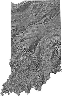
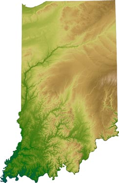
The four Tagged Image File Format (TIFF) images shown in Figure 4 are samples of graphical images that were created from the new statewide DEM using ArcView 3.3 and desktop publishing software. To create these images the following procedure was used. First, the grid was imported into ArcView using the Spatial Analyst extension and a color ramp was applied. Second, the hillshade was created with the surface\hillshade option. Finally, the graphical images were created and exported using an extension called Image Conversion-Georeferencing2, adapted from a script by Kenneth McVay (downloadable from ESRI’s ArcScripts website at http://arcscripts.esri.com/details.asp?dbid=10603). This extension exports images of several file formats while maintaining original raster resolution and also creates a world file. Images may be exported as color DEMs, hillshades, or a combination of both DEM and hillshade.

A		B
C		D
Figure 4. Thumbnails of TIFF images made from the new DEM—available on CD-ROM by Brown and others (2004). Image of the colored DEM only. A color ramp was applied to the DEM in ArcView 3.3. Image of the grayscale hillshade only. Combined image of the colored DEM and the hillshade, exported from ArcView as one image. Combined image of the colored DEM and the hillshade which were exported from ArcView individually (Figure 4A and 4B). The two images were placed into Adobe Illustrator as separate layers where they were combined and enhanced.

Once the images are exported as TIFFs, they may be imported into graphics software programs such as Adobe Illustrator with the Avenza MAPublisher filter, where georegistered TIFFS may be added as layers with their world files. The MAPublisher filter allows for on-screen data analysis and for creating new GIS information. Further enhancements can be accomplished in Adobe Photoshop where various adjustments can illuminate textures and patterns not usually visible. Resultant images can be returned to any GIS application, with their original world files.

CREDITS

The IGS purchased the NED from the USGS with funds from a 319 grant from the Indiana Department of Environmental Resources (IDEM). The 1:24,000-scale hypsography was provided to the IGS by the Indiana Department of Natural Resources (INDR), which received them from the USGS. Chris Dintaman, IGS geologist and GIS analyst, standardized a set of commands and variables within ArcInfo to produce the new DEMs.

REFERENCES

Berry, G.M., Bleuer, N.K., Brown, S.E., Dickson, M.L., Dintaman, C., Olejnik, J., and Rupp, R., 2004, Surface Terrain of Indiana: Indiana Geological Survey Poster, POSTER05, accessed at http://igs.indiana.edu/survey/publications/searchPubsDetail.cfm?Pub_Num=POSTER05.

Brown, S.E., Bleuer, N.K., Dickson, M., Dintaman, C., Olejnik, J., and Rupp, R., 2004, Digital Elevation Model of Indiana—Revised: Indiana Geological Survey Open-File Studies, OFS04-01, accessed at http://igs.indiana.edu/survey/publications/searchPubsDetail.cfm?Pub_Num=ofs04-01.

APPENDIX

1. Obtain 1:24,000 DLG hypsography from the USGS.
2. Check each attribute table in each hypsography file for the number of major and minor fields; there can be 4 pairs or more of major/minor fields depending on the amount of information conveyed. The elevation values are located in the minor fields. In ArcInfo, use the APPEND command to group the DLGs by similar number of major and minor fields (group those with major3 and minor3 together, those with major4 and minor4 together, etc.).
3. In ArcInfo Tables, use ADDITEM command to add a field called ELEV to the attribute table for each DLG. Then populate the ELEV field with the elevation values from the minor fields. Use the DROPITEM command to delete the data columns labeled major and minor.
4. Delete unnecessary “boundary” arcs—those with ELEV values of 0. Also, delete arcs with ELEV values of 5, 10, 15, etc, if these are obviously not elevations. These are usually lake-bottom depths.
5. Append all the edited DLG coverages into one coverage. Build this coverage in ArcInfo for lines, but not for polygons.
6. Obtain USGS hydrography, if available. If USGS hydrography is not available, obtain U.S. Census Bureau lake and stream data.
7. Use the geoprocessing wizard in ArcView to merge all the stream shapefiles and the waterbody shapefiles together to make a seamless shapefile of the entire area. Delete all double-edged streams and very small lakes in the waterbody shapefile (if using TIGER files). Delete all arcs around all lakes in the stream shapefile (there should be no lakes on the stream coverage). Redigitize any lines that are missing after deleting the lakes in stream valleys. All double-edged streams should be redigitized down the center of the valley.
8. Convert the waterbody shapefiles and the stream shapefiles to coverages in ArcInfo. Then build the water body coverage for polygons and the stream coverage for lines.
9. Edit the stream flow directions in ArcEdit so that each segment of each stream has the proper flow direction. This process can be labor intensive, as many of the stream flow directions are reversed.
10. Run the TOPOGRID command in ArcInfo GRID using the following list of subcommands and parameters:
    
    <Arc command prompt>: topogrid grid_name 30 (the grid to be created and the cell size, in map units, of the output grid)
    TopoGrid: contour coverage_name elev (keyword and parameters for input of a line coverage representing elevation contours; this command causes ArcInfo to prompt the user for the keywords and parameters)
    TopoGrid: datatype contour (the primary type of input data)
    TopoGrid: enforce on (enforce trends of drainage)
    TopoGrid: iterations 30 (maximum number of iterations for the resolution)
    TopoGrid: outputs sink_1 drain_1 diag_1 (optional outputs providing information that can be used to evaluate the output elevation grid)
    TopoGrid: stream stream_name (keyword for input of a line coverage representing streams)
    TopoGrid: lake lake_name (keyword for input of a polygon coverage representing lakes)
    TopoGrid: tolerances 2.5 1 0 (a set of tolerances used to adjust the calculations of the interpolation and drainage enforcement process)
    TopoGrid: end
11. Clip the resulting grid to a buffered shapefile (the outline of the new DEMs with a 1,000-meter buffer).
12. Merge the final clipped grid or grids back into the state DEM using the ArcInfo MERGE command in GRID—grid: final_name = merge (1stpriorityclip, 2ndprioritystate, etc).
13. Change the type of grid from a floating point grid to an integer grid. This creates a much smaller file.