U.S. Geological Survey Open-File Report 2005-1428
Digital Mapping Techniques '05—Workshop Proceedings
Earth Sciences Sector Contribution No. 2005148
Surficial geology mapping at the Geological Survey of Canada (Atlantic) or GSCA, has gone through several revolutions since inception in the early 1970s. Then, extensive mapping was based on echo sounder data, complemented by data from low-resolution sub-bottom profiling systems and sidescan sonar systems. The advent of high-resolution sub-bottom profilers (e.g., the Huntec DTS, or Deep-Towed System) augmented the suite of tools available to marine geologists.
The standard outcomes of the work completed between the 1970s and the mid 1990s were surficial geology maps, accompanied by reports. These maps commonly allocated areas of the sea floor to one of a number of formations (e.g., Scotian Shelf Drift Formation). Workers uncomfortable with the formation concept used genetic schema which had similar outcomes. For example, a regional equivalent of the Scotian Shelf Drift Formation was mapped as ice-contact sediment.
The advent of multibeam bathymetry mapping in the mid-1990s provided geologists with images of the sea floor that had unprecedented clarity. From the beginning, multibeam bathymetric data have been portrayed in different formats at various scales, perhaps reflecting the absence of a systematic offshore mapping program. The advent of mapping of larger areas, allied with the possible advent of systematic mapping involving collaboration between GSCA and the Department of Fisheries and Oceans (DFO) (similar to the collaboration involving echo sounder data in the 1970s), revealed a pressing need for a more systematic approach to the content and appearance of multibeam imagery, and in particular, standardization of the types of maps produced (Shaw and Todd, 2003).
Multibeam bathymetric survey techniques used in the St. Georges Bay area (Figure 1) provide a rapid means of determining the morphology and nature of the sediments on the seafloor (Figure 2). A multi-element transducer provides many (30-150) individual soundings of the water depth and echo strength for each ping. Automatic seafloor tracking programs determine depths and echo strengths for each transducer element, correct for transducer motion, and calculate a geographic co-ordinate for each individual sounding.
A wide swath (up to 7 times the water depth) can be surveyed in a single pass through an area. Survey lines are spaced to provide overlapping coverage of the seafloor. The data are used to generate high-resolution images that contain information about the morphology of the seabed.
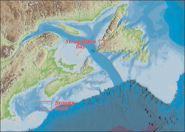
Figure 1. Location map showing two sample map areas, St Georges Bay and Browns Bank (from Shaw and Courtney, 2004).
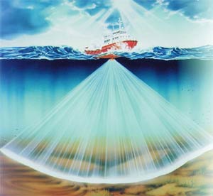
Figure 2. Multibeam bathymetric survey techniques provide a rapid means of determining the morphology and nature of the sediments on the seafloor. A wide swath (up to 7 times the water depth) can be surveyed in a single pass through an area (used with permission of Kongsberg Simrad).
The sun-illuminated DEM of bathymetry (Figure 3) is based on a GEOTIFF exported from the GSCA GRASS software. Many analysts prefer grey-scale images for detection of morphologic features on the sea floor, arguing that colour can mask variability. Commonly, hot-to-cold colour ramps are used (also referred to as rainbow colour ramps). In this scheme, blue is used to represent the deep areas, green the intermediate depths, and red the shoals. Some problems arise concerning the range of depth values represented by individual colour bands. Since the inception of multibeam processing at GSCA, the rainbow scheme has been used to represent depth. When a colour bar is applied in the GRASS software, the rainbow scheme is automatically used.
In many multibeam bathymetry map areas, much of the bathymetry variation is in a narrow band. For example, on the Scotian Shelf banks, the predominant depth may be 100-110 m while intervening basins and troughs may be 200-300 m deep. However, if colours are selected automatically, all depths on the bank might be allocated the same shade of red, and this obscures important morphologic variability. It would be preferable to have the subtle depth variations on the bank highlighted by allowing greater colour variation over the 100-110 m interval, for example from red to green. Colour distribution optimization can be achieved by first determining the hypsometric frequency of the data and then tuning the colour bar accordingly.
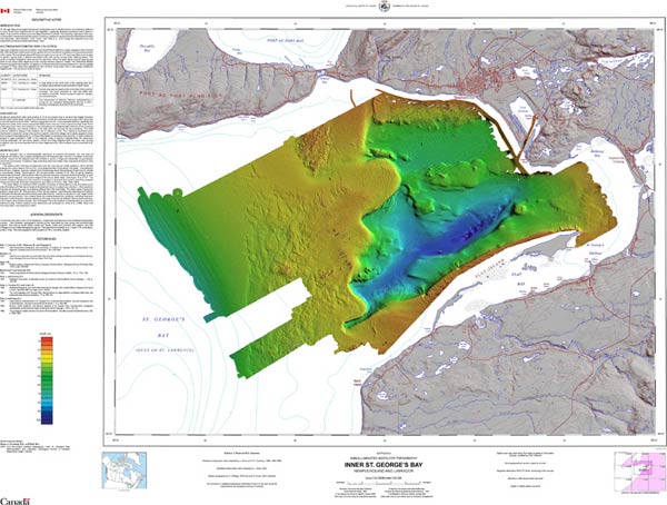
Figure 3. Bathymetry map—the sun-illuminated DEM of bathymetry is based on a GEOTIFF exported from the GSCA GRASS software. Depth is represented by colour. Additional information includes isobaths (contours of depth), a representation of land areas, and isobaths from Canadian Hydrographic Service nautical charts. In the printed version of the Proceedings, these figures are in black and white; however, the web version shows these figures in full colour.
GSC has traditionally represented backscatter on a grey scale. The usual practice has been to portray areas of high backscatter (commonly gravel and rock) as dark tones, and to portray areas of low backscatter (sand and mud) as light tones (Figure 4). This approach parallels the customary depiction of the sea floor on sidescan sonograms: areas of high reflectivity (gravel, rock, shipwrecks etc.) have dark returns, whereas muddy and sandy sea floors with low reflectivity have light returns. The inverse approach is used by University of New Brunswick Ocean Mapping Group, who commonly depict mud as dark-toned. There are no advantages of one method over the other: it is mostly a matter of personal preference, in which those accustomed to examining sidescan sonograms prefer the first option, However, backscatter is also very effectively represented using colour (Figure 4).
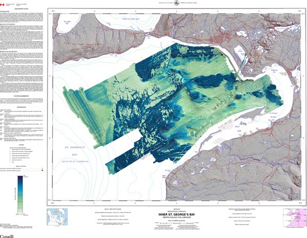
Figure 4. Backscatter mapbackscatter is very effectively represented using colour. Here an indigo to pale green colour scheme is applied, so that indigo represents high backscatter and pale grey represents low backscatter. There are also some advantages to draping the coloured backscatter over the sun-illuminated topography.
This map (Figure 5) is the vehicle for an interpretation of the imagery. We take the shaded relief imagery and explain what is seen in terms of geological processes. In other words, it is the opportunity to turn information into knowledge, with several approaches possible:
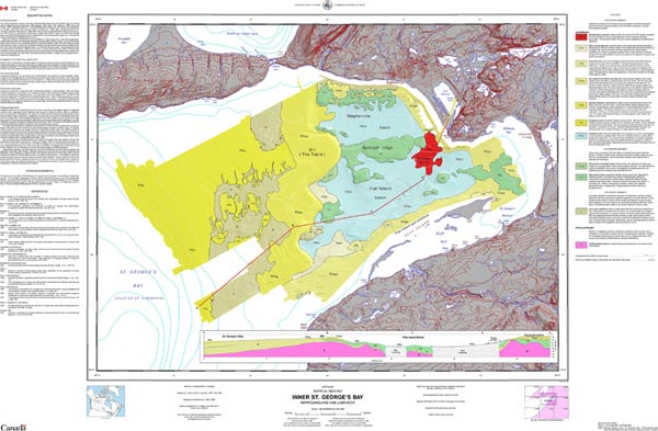
Figure 5. Surficial Geology map—this map shows how the shaded relief imagery is used and explains what is interpreted in terms of geological processes.
Based on the sea floor sediment maps and statistical analyses of benthos (Figure 6), habitats and corresponding associations of benthic animals are mapped. In the case of the Browns Bank habitat map, each of the habitats is distinguished on the basis of substrate, habitat complexity, relative current strength and water depth. Different locations may require utilization of other information to distinguish habitats. The spatial allocation of samples, and abundance and commonness of species are used as additional guidelines for identification of habitat zonation.
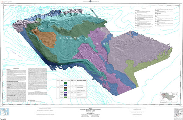
Figure 6. Benthic habitat map—based on the sea floor sediment maps and statistical analyses of benthos, habitats and corresponding associations of benthic animals are mapped.
The aim of this symbol set (Figure 7) is to promote symbol design and usage which will help to eliminate confusion and inconsistency on published maps, as well as promote a more quantitative definition of interpreted information.
A large volume of marine geological data has accumulated worldwide over the last number of decades and has stimulated the publication of large numbers of interpreted marine geological maps. While the raw data for these interpretations may derive from numerous sourcesgovernment surveys, the offshore oil and gas industry, the offshore mining industryit has generally been the task of government agencies to compile and synthesize the information into map form. A characteristic of marine geological maps, particularly those representing aspects of the surficial geology, is the diversity not only of the symbols used to represent features or zonations, but also in the levels of interpretation implied by those symbols. For example, where one worker may use an S to denote only the occurrence of scouring on the seabed, another may mark the location with an X varying in size according to the typical scour width, and qualified by an adjacent number indicating scour density at that location of depth of scour. Reconciliation of these approaches is not only frustrated by the difference in representative symbols, but also in the amount of information conveyed (Fader and Peters, 1988).
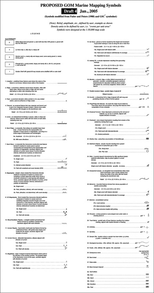
Figure 7. Marine mapping symbol set—the goal of this symbol set is to promote use of symbol design, which will help to eliminate confusion and inconsistency on published maps, as well as promote a more quantitative definition of interpreted information.
The new policy of Geological Survey of Canada is to provide free, on-line access to all new map products (Figure 8). When completed these maps will become part of the national Geoscience Data Repository (GDR), a collection of geoscience databases managed by a series of standardized Information Services (http://gdr.nrcan.gc.ca/). The aim of the GDR is to standardize corporate geoscience databases and make them interoperable in order to increase the discovery, access, and use of the information that the GSC has been mandated to collect and maintain. The maps will be available on-line as printable image files (PDF, MrSid), and digital GIS layers accessible through Open Geospatial Consortium (OGC) standards such as Web Map Service or WMS.
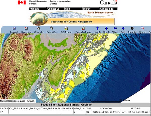
Figure 8. Online access to the map products—the policy of Geological Survey of Canada is to provide free, online access to all new map products. When completed, these maps will become part of the national Geoscience Data Repository (GDR), a collection of geoscience databases managed by a series of standardized Information Services (http://gdr.nrcan.gc.ca/).
GSC A-series maps are maps that are subject to critical review by at least one scientific authority. They are multicoloured maps printed on demand on colour ink jet plotters or on quality stock when large pres-runs of several hundred copies are needed. A-series maps are also available in digital format on CD-ROMs and even, in some cases, released on the Internet. Instructions on database standards and procedures for geological map production are available on the Internet at http://www.nrcan.gc.ca/ess/carto/specifications_e.html.
Bathymetry Map (Figure 3): The sun-illuminated DEM of bathymetry is based on a GEOTIFF exported from the GSC (Atlantic) GRASS (GIS) software. Depth is represented by colour. The DEMs Geographic projection, datum, etc are made to match the base map at the time of importing (via Add Data) in ArcMap.
Backscatter Map (Figure 4): High backscatter (high reflectivity-gravel rock, etc.) is represented by indigo blue and low backscatter (low reflectivity-mud, etc.) by the pale grey/green. The backscatter values are draped over the greyscale multibeam bathymetry.
Surficial Geology Map (Figure 5): The interpretation of surficial geology is shown as coloured polygons that are draped over a greyscale map of the multibeam bathymetry. The geological data polygon boundaries can be as acquired by heads-up digitizing, in ArcMap on a separate layer with the backscatter duotone underneath as the guide to accurately digitizing the features. A second method can also be used; this is making a hard copy print of the backscatter and overlaying it with a sheet of translucent mylar (plastic). With the mylar taped securely to the backscatter duotone print, the outline for the geological features can be traced with a black ink technical pen or a fine tip marker. This overlay is then scanned, put through ArcScan to vectorize the polygon boundaries and with the latitude and longtitude control points is now added (rubbersheeted) as data (in a feature class) to ArcMap.
Benthic Habitat Map (Figure 6): Benthic habitat interpretation polygons were draped over a greyscale multibeam bathymetry of the mapped area and were compiled in the same way as in Figure 5 and then added to ArcMap.
For the land area a greyscale DEM was used as an underlay to the culture, drainage, etc. The greyscale DEM was derived from processing the elevations of the topographic contours layer. To allow the overlay, culture, drainage, etc., data to be viewed clearly, a transparency value is applied to the greyscale DEM; in most cases a value of 50% is adequate.
The map border, at present, is made in the GSCs Geological Mapping System GEMS routine, (via Create Border), in ArcInfo. The border is produced as an ArcInfo Coverage, complete with coordinate text, ticks, neatline, etc. This border coverage is added to the map folder in ArcCatalogue and then the border arc file and polygon file are saved into an ArcMap feature class/feature dataset, the same is done for the neatline and coordinate annotations.
Once the border is made to the required map extents (map area), then the base data is added, this data can be acquired from the National Topographic DataBase (NTDB) topo maps data library, Geomatics Canada, Ottawa www.cits.rncan.gc.ca. These data layers, topographic contours, drainage, culture and annotations can be added as an arc, node or annotation in a feature class. If the personal geodatabase for the map is set up correctly, then the feature class is inside a feature dataset that is inside the personal geodatabase (i.e. personal geodatabasefeature datasetfeature class, this is how these three items are seen in ArcCatalogue and ArcMap Table Of Contents). The personal geodatabase should be the first thing set up when a new map is started.
These file structure/management issues are usually addressed in ArcCatalogue and then added (via Add Data) to ArcMap. There is a third ArcGIS tool usedArcToolbox, an ArcGIS module that is used for file conversion, analysis and data management; the functions include Analysis (surface-cut and fill), Conversion (Import to Geodatabase), Data Management (Projections-Spatial adjustment or rubbersheeting).
The Location map (a small map of Canada and its offshore) for A-Series maps is now a layer (linked through a database at GSC (Ottawa) via the internet) that can be added to ArcMap (via Add Data). The location dot, (the study area), of the map is linked to the neatline of the map being drawn.
At this time, the National Topographic System (NTS) index map is not linked to the GSC database (Ottawa). It is made in the GEMS routine, (via Create NTS Index Map) and output as a .eps file from ArcInfo, imported to CorelDraw and placed in the ArcMap map surrounds as a linked graphic.
The surround text, (descriptive notes, references, title blocks, etc.) are created in CoreDraw and imported to ArcMap (via Insert-Object) as graphic elements that are linked files to CoreDraw. This ArcMap/CorelDraw linking allows edits to be done in CorelDraw and will automatically update the ArcMap element. Other graphic software can be used such as Macromedia Freehand and Illustrator. All the placements of cartographic elements and data in the surrounds and on the map area use the GSCs cartography specs. For A-series maps, these specifications are found at http://ess.nrcan.gc.ca/pubs/carto/specifications_e.php.
Shaw, John and Todd B.J., 2003, Development of mapping standards for marine bathymetry, backscatter, geology and habitat maps: Geological Survey of Canada internal report, p. 1-22.
Fader, B.J.G., and Peters, J., 1988, Symbols for mapping of marine surficial geological features. Federal Geographic Data Committee (FGDC), digital cartographic standard for geologic map symbolization: Geological Survey of Canada internal report, p.1-16.
Shaw, J., and Courtney, R.C., 2004, A digital elevation model of Atlantic Canada: Geological Survey of Canada Open File Report 4634, Compact Disk.

![]() U.S. Department of the Interior |
U.S. Geological Survey
U.S. Department of the Interior |
U.S. Geological Survey
URL: pubsdata.usgs.gov /pubs/of/2005/1428/grant/index.html
Page Contact Information: David R. Soller
Page Last Modified: Saturday, 12-Jan-2013 22:04:53 EST
