NORTHPORTALL_RESBELOWSED.SHP: Processed continuous resistivity profile (CRP) data below the sediment water interface from Northport Harbor on Long Island, New York collected from May 12 to May 14, 2008

Metadata also available as - [Outline] - [Parseable text]

Frequently-anticipated questions:


What does this data set describe?

Title:
NORTHPORTALL_RESBELOWSED.SHP: Processed continuous resistivity profile (CRP) data below the sediment water interface from Northport Harbor on Long Island, New York collected from May 12 to May 14, 2008
Abstract:
An investigation of coastal groundwater systems was performed along the north shore of Long Island, New York during May 2008 to constrain nutrient delivery to Northport Harbor and Manhasset Bay by delineating locations of likely groundwater discharge. The embayments are bounded by steep moraines and are underlain by thick fine-grained sediments deposited in proglacial lakes during the last ice age. Beach sand and gravel overlie the glacial deposits along the coast. The continuous resistivity profiling (CRP) surveys that were conducted indicate the existence of low-salinity groundwater in shore-parallel bands, typically 25 to 50 meters wide, along the shorelines of both bays. Piezometer sampling and seepage meter deployments in intertidal and subtidal areas of the two bays confirmed the presence and discharge of brackish and low-salinity groundwater. The large tidal ranges (up to 3 meters), and the steep onshore topography and hydraulic gradients are important variables controlling coastal groundwater discharge in these areas. For more information on the survey involved in this project, see <http://quashnet.er.usgs.gov/data/2008/08007/>.
  1. How should this data set be cited?

    Bratton, John F. , and Cross, VeeAnn A. , 2012, NORTHPORTALL_RESBELOWSED.SHP: Processed continuous resistivity profile (CRP) data below the sediment water interface from Northport Harbor on Long Island, New York collected from May 12 to May 14, 2008: Open-File Report 2011-1041, U.S. Geological Survey, Coastal and Marine Geology Program, Woods Hole Coastal and Marine Science Center, Woods Hole, MA.

    Online Links:

    This is part of the following larger work.

    Cross, V.A., Bratton, J.F., Crusius, J., Kroeger, C.W., and Worley, C.W., 2012, Continuous Resistivity Profiling Data from Northport Harbor and Manhasset Bay, Long Island, New York: Open-File Report 2011-1041, U.S. Geological Survey, Coastal and Marine Geology Program, Woods Hole Coastal and Marine Science Center, Woods Hole, MA.

    Online Links:

    Other_Citation_Details: CD-ROM

  2. What geographic area does the data set cover?

    West_Bounding_Coordinate: -73.366910
    East_Bounding_Coordinate: -73.353150
    North_Bounding_Coordinate: 40.911388
    South_Bounding_Coordinate: 40.888438

  3. What does it look like?

    <https://pubs.usgs.gov/of/2011/1041/data/resistivity/shapefile/northportall_resbelowsed.gif> (GIF)
    Thumbnail GIF image showing the location of the processed CRP data in Northport Harbor. The coastline with piers is included for spatial reference.

  4. Does the data set describe conditions during a particular time period?

    Beginning_Date: 12-May-2008
    Ending_Date: 14-May-2008
    Currentness_Reference: ground condition

  5. What is the general form of this data set?

    Geospatial_Data_Presentation_Form: vector digital data

  6. How does the data set represent geographic features?

    1. How are geographic features stored in the data set?

      This is a Vector data set. It contains the following vector data types (SDTS terminology):

      • Entity point (272645)

    2. What coordinate system is used to represent geographic features?

      Horizontal positions are specified in geographic coordinates, that is, latitude and longitude. Latitudes are given to the nearest 0.000001. Longitudes are given to the nearest 0.000001. Latitude and longitude values are specified in Decimal degrees.

      The horizontal datum used is D_WGS_1984.
      The ellipsoid used is WGS_1984.
      The semi-major axis of the ellipsoid used is 6378137.000000.
      The flattening of the ellipsoid used is 1/298.257224.

      Vertical_Coordinate_System_Definition:
      Depth_System_Definition:
      Depth_Datum_Name: Local surface
      Depth_Resolution: 0.1
      Depth_Distance_Units: meters
      Depth_Encoding_Method: Explicit depth coordinate included with horizontal coordinates

  7. How does the data set describe geographic features?

    northportall_resbelowsed
    ESRI point shapefile (Source: ESRI)

    FID
    Internal feature number. (Source: ESRI)

    Sequential unique whole numbers that are automatically generated.

    Shape
    Feature geometry. (Source: ESRI)

    Coordinates defining the features.

    ID
    An automatically generated numeric value. (Source: Avenue script.)

    Range of values
    Minimum:0
    Maximum:0

    DIST
    Distance along the line in meters. Originally calculated by the AGI processing software. (Source: Software calculated.)

    Range of values
    Minimum:0.1
    Maximum:2507.3
    Units:meters

    LONGITUDE
    Longitude position of the point (decimal degrees, WGS84) (Source: U.S. Geological Survey - calculated by the avenue script used to process the data.)

    Range of values
    Minimum:-73.36691
    Maximum:-73.35315
    Units:decimal degrees

    LATITUDE
    Latitude position of the point (decimal degrees, WGS84) (Source: U.S. Geological Survey - calculated by the avenue script used to process the data.)

    Range of values
    Minimum:40.888438
    Maximum:40.911388
    Units:decimal degrees

    UTMX
    Easting position of the point in meters (UTM, Zone 18, WGS84) (Source: U.S. Geological Survey - calculated by the avenue script used to process the data.)

    Range of values
    Minimum:637540.2
    Maximum:638720.3
    Units:meters

    UTMY
    Northing position of the point in meters (UTM, Zone 18, WGS84) (Source: U.S. Geological Survey - calculated by the avenue script used to process the data.)

    Range of values
    Minimum:4527663.3
    Maximum:4530216.3
    Units:meters

    DEPTH
    Depth (meters) of the resistivity value below the water surface (not tide corrected - local surface). (Source: Acquisition/processing software derived.)

    Range of values
    Minimum:-12.32
    Maximum:-0.3
    Units:meters

    DEP_B_SED
    Depth (meters) of the value below the sediment/water interface. (Source: Processing software derived (MATLAB - justbelowsed.m).)

    Range of values
    Minimum:-12.02
    Maximum:0
    Units:meters

    RESVALUE
    Resistivity value of the data point in ohm-m. (Source: Processing software calculated (AGI EarthImager).)

    Range of values
    Minimum:0.100366
    Maximum:506.016
    Units:ohm-m

    RESLOGVAL
    Log(10) of the resistivity value. (Source: Processing software calculated (MATLAB justbelowsed.m).)

    Range of values
    Minimum:-0.998413
    Maximum:2.704164
    Units:Log(10) of ohm-m

    LINE
    The alphanumeric name corresponding to the individual line of data collection that the point comes from. (Source: U.S. Geological Survey)

    Character set.


Who produced the data set?

  1. Who are the originators of the data set? (may include formal authors, digital compilers, and editors)

  2. Who also contributed to the data set?

  3. To whom should users address questions about the data?

    VeeAnn A. Cross
    U.S. Geological Survey
    Marine Geologist
    Woods Hole Coastal and Marine Science Center
    Woods Hole, MA 02543-1598

    (508) 548-8700 x2251 (voice)
    (508) 457-2310 (FAX)
    vatnipp@usgs.gov


Why was the data set created?

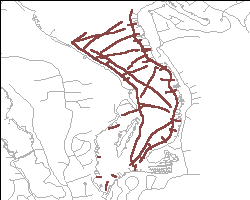
The purpose of this dataset is to release in shapefile format all the processed continuous resistivity profile data that occurs at the sediment water interface or below collected in Northport Harbor on Long Island, New York from May 12 - May 14, 2008. Additionally, the release of these data acts as a data archive.


How was the data set created?

  1. From what previous works were the data drawn?

    (source 1 of 1)
    Source_Contribution:
    The continuous resistivity profile (CRP) system used on this cruise was an AGI SuperSting marine system described at the website: www.agiusa.com/marinesystem.shtml. Two different streamers were used for data collection - not simultaneously. One streamer was a 50-m streamer with an 11 electrode array with electrodes spaced 5 meters apart. The other streamer was a 15-m streamer with an 11 electrode array with electrodes spaced 1.5 meters apart. In both cases, the source electrodes are graphite, while the receiver electrodes are stainless steel. A dipole-dipole configuration was used for the data collection in which two fixed current electrodes are assigned with the measurement of voltage potential between electrode pairs in the remaining electrodes. The maximum depth below the water surface the streamer can reach is approximately ¼ the streamer length. So for the 50-m streamer, maximum depth is about 12.5 meters, while the 15 meter streamer can reach about 3.75 meters. Each line of data acquisition records several files. The two files necessary for processing are the *.stg and the *.gps file. The STG file contains the resistivity data, while the GPS file contains the navigation information. The navigation system used in concert with the CRP system is a Lowrance LMS-480M with an LGC-2000 GPS antenna and a 200 kHz fathometer transducer. The transducer also contains a temperature sensor. Lowrance indicates the speed of sound used by the system is 4800 feet/second. Both the temperature and depth information are recorded in the logged GPS file. The CRP system images the subsurface electrical properties of an estuarine, riverine or lacustrine environment. Resistivity differences can be attributed to subsurface geology (conductive vs less conductive layers) and hydrogeologic conditions with fresh water exhibiting high resistivity and saline conditions showing low resistivity.

  2. How were the data generated, processed, and modified?

    Date: Sep-2008 (process 1 of 5)
    A MATLAB script (justbelowsed.m) was run on the processed CRP files to generate files with just the resistivity values that fall below the sediment water interface, and an extrapolated value at the sediment water interface. Two files from the processed resistivity data are needed for this script: the XYZ output from the EarthImager processing which has distance along line (meters), depth of resistivity reading (meters), and resistivity value (ohm-m); and the DEP file that contains distance along line (meters) and water depth values (meters). Because some lines are short and don't require a "roll-along" processing technique, the XYZ information is contained in a file with the DAT extension. The MATLAB script combines the two data files (processed resistivity and depth files) such that the output is only the resistivity values that fall at or below the sediment water interface. This script was written by the USGS (VeeAnn A. Cross) in Woods Hole, MA. In order to have a resistivity value at the sediment water interface, the software usually has to interpolate resistivity values. The version of MATLAB used for these data was MATLAB 7.5.0.342 (R2007b). An example of the script usage in MATLAB is: justbelowsed('L10F1_lin_AllInvRes.xyz','L10F1_lin_wres.dep') The output is: L10F1_lin_AllInvRes_jbsed.xyz This resulting XYZ file has 5 columns of information: distance along line (meters); depth below water surface (meters); depth below sediment/water interface (meters); resistivity value (ohm-m); log(10) resistivity value. This process step and all subsequent process steps were performed by the same person - VeeAnn A. Cross.

    Person who carried out this activity:

    VeeAnn A. Cross
    U.S. Geological Survey
    Marine Geologist
    Woods Hole Coastal and Marine Science Center
    Woods Hole, MA 02543-1598

    (508) 548-8700 x2251 (voice)
    (508) 457-2310 (FAX)
    vatnipp@usgs.gov

    Data sources used in this process:
    • *.xyz or *.dat
    • *.dep

    Data sources produced in this process:

    • *_jbsed.xyz

    Date: Sep-2008 (process 2 of 5)
    Using ArcView 3.3 and the avenue script resist_jbsed_nan.ave (script written by VeeAnn Cross at the USGS in Woods Hole, MA) these XYZ files are converted to shapefiles. This script requires that the navigation for the resistivity line be a polyline shapefile and present in the view. The script prompts the user for the polyline shapefile in the view that they want to use, then prompts the user to browse for the xyz resistivity file. The script then creates a new point shapefile, with a point along the polyline at each value of X specified in the xyz file. The y and z values, as well as longitude and latitude are added to the point shapefile. This requires that the view be projected, as the distance in the xyz file is in meters. This script will work on a single line polyline shapefile (ie the nav for a survey line is alone in a shapefile) or on a selected line within a polyline shapefile. The result is a point shapefile with 11 columns of information. The Id attribute is automatically generated upon creation of a shapefile, the line attribute is the line name as indicated within the polyline shapefile that the program prompts the user for, dist is the distance along attribute carried over from the MATLAB file, the attributes of location information (latitude, longitude, utmx, utmy) are calculated by the tool, the attributes depth, dep_b_sed, resvalue, and reslogval are carried over from the MATLAB file. The Entity and Attribute section further describes these attributes and their units. This particular script had to handle NaN values generated by MATLAB where the CRP data only contained information in the water column because the water was too deep for the resistivity streamer to penetrate the sediment water interface. ***A problem detected much later with L36F2 on day 3 required the jbsed shapefile for that line to be recalculated. This calculation was performed in ArcMap 9.2 using VAC Extras (an ArcMap extension written by the USGS in Woods Hole). Using VAC Extras, version 2.1 - VAC Extras - Resistivity - convert resistivity to shapefile. This program performs the exact same function as the ArcView 3.3 avenue script. The one exception is the attributes are in a slightly different order. The fix to L36F2 occurred in February, 2011.

    Data sources used in this process:

    • *_jbsed.xyz
    • the polyline shapefiles for individual days of data collection

    Data sources produced in this process:

    • all the point shapefiles for each individual line.

    Date: Sep-2008 (process 3 of 5)
    Then using the geoprocessing extension that comes with ArcView 3.3, the individual point shapefiles for each line of collection were merged into a single point shapefile for each day of collection. ***Because of a problem discovered with L36F2, the day3 resbelowsed shapefiles had to be remerged. Day 3 was merged using ArcMap 9.2 - ArcToolbox - Data Management Tools - General - Merge. Even though L36F2 has attributes in a slightly different order, all the same attributes are present, so the attribute mapping was left to the default. This merge occurred Feb. 2011.

    Data sources used in this process:

    • individual point shapefiles for each line of collection

    Data sources produced in this process:

    • day1all_resbelowsed.shp
    • day2all_resbelowsed.shp
    • day3all_resbelowsed.shp

    Date: Sep-2008 (process 4 of 5)
    Using ArcMap 9.2 - ArcToolbox - Data Management Tools - Projections and Transformations - Define Projection define the projection of the point shapefiles from day1 and day2 as Geographic, WGS84. Because of the reprocessing of day 3 in 2011, that shapefile did not need to have the projection defined.

    Data sources used in this process:

    • day1all_resbelowsed.shp
    • day2all_resbelowsed.shp

    Data sources produced in this process:

    • day1all_resbelowsed.shp
    • day2all_resbelowsed.shp

    Date: Feb-2011 (process 5 of 5)
    Combine the individual days of the resbelowsed files into a single shapefile. Within ArcMap 9.2, using ArcToolbox - Data Management Tools - General - Merge input files: day1all_resbelowsed, day2all_resbelowsed, day3all_resbelowsed; output: northportall_resbelowsed.shp. Left field mapping at the defaults.

    Data sources used in this process:

    • day1all_resbelowsed.shp
    • day2all_resbelowsed.shp
    • day3all_resbelowsed.shp

    Data sources produced in this process:

    • northportall_resbelowsed.shp

  3. What similar or related data should the user be aware of?


How reliable are the data; what problems remain in the data set?

  1. How well have the observations been checked?

  2. How accurate are the geographic locations?

    The navigation system used was a Lowrance 480M with an LGC-2000 Global Positioning System (GPS) antenna. The antenna was located at the anchor point for the resistivity streamer, which is also directly above the fathometer transducer mount point. The GPS system is published to be accurate to within 10 meters.

  3. How accurate are the heights or depths?

    All bathymetry values were collected by the 200 kHz Lowrance fathometer. The fathometer was mounted starboard side aft, directly below the GPS antenna and the resistivity streamer tow point. The transducer was approximately 0.30 meters below the sea surface, and this draft was not corrected for. The Lowrance manufacturer indicates the speed of sound used by the system to convert to depths is 4800 feet/second (1463 meters/second). All values are assumed to be accurate to within 1 meter.

  4. Where are the gaps in the data? What is missing?

    This shapefile represents all the CRP data collected at this location from the sediment water interface and deeper. In some cases the water depth was too great for the system - the sediment wasn't penetrated. Therefore no values exist in those locations.

  5. How consistent are the relationships among the observations, including topology?

    All of the processed CRP data were handled in the same way.


How can someone get a copy of the data set?

Are there legal restrictions on access or use of the data?

Access_Constraints: None.
Use_Constraints:
The public domain data from the U.S. Government are freely redistributable with proper metadata and source attribution. Please recognize the U.S. Geological Survey as the originator of the dataset.

  1. Who distributes the data set? (Distributor 1 of 1)

    VeeAnn A. Cross
    U.S. Geological Survey
    Marine Geologist
    Woods Hole Coastal and Marine Science Center
    Woods Hole, MA 02543-1598

    (508) 548-8700 x2251 (voice)
    (508) 457-2310 (FAX)
    vatnipp@usgs.gov

  2. What's the catalog number I need to order this data set?

    Downloadable Data

  3. What legal disclaimers am I supposed to read?

    Neither the U.S. government, the Department of the Interior, nor the USGS, nor any of their employees, contractors, or subcontractors, make any warranty, express or implied, nor assume any legal liability or responsibility for the accuracy, completeness, or usefulness of any information, apparatus, product, or process disclosed, nor represent that its use would not infringe on privately owned rights. The act of distribution shall not constitute any such warranty, and no responsibility is assumed by the USGS in the use of these data or related materials. Any use of trade, product, or firm names is for descriptive purposes only and does not imply endorsement by the U.S. Government.

  4. How can I download or order the data?

  5. What hardware or software do I need in order to use the data set?

    This WinZip file contains data available in ESRI point shapefile format. The user must have software capable of uncompressing the WinZip file and reading/displaying the shapefile.


Who wrote the metadata?

Dates:
Last modified: 12-Jan-2012
Metadata author:
VeeAnn A. Cross
U.S. Geological Survey
Marine Geologist
Woods Hole Coastal and Marine Science Center
Woods Hole, MA 02543-1598

(508) 548-8700 x2251 (voice)
(508) 457-2310 (FAX)
vatnipp@usgs.gov

Metadata standard:
FGDC Content Standards for Digital Geospatial Metadata (FGDC-STD-001-1998)
Metadata extensions used:


Generated by mp version 2.9.6 on Thu Jan 12 17:16:46 2012