
![]()
U.S. GEOLOGICAL SURVEY
Scientific Investigations Report 2004–5237
Conceptual Model and Numerical Simulation of the Ground-Water-Flow System in the Unconsolidated Deposits of the Colville River Watershed, Stevens County, Washington
Numerical Simulation of the Ground-Water-Flow System
Development of a numerical model allows for a detailed analysis of the movement of water through the hydrogeologic units that constitute the ground-water-flow system. Ground-water flow in the unconsolidated deposits of the Colville River Watershed was simulated using the U.S. Geological Survey modular three-dimensional finite-difference ground-water-flow model, MODFLOW-2000 (Harbaugh and others, 2000).
Model Description
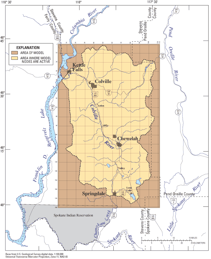
The MODFLOW program uses data sets that describe the hydrogeologic units, recharge, discharge, and conceptual model of the ground-water-flow system, and calculates hydraulic heads at discrete points (nodes) and flow within the model domain. The program requires that the ground-water-flow system be subdivided, vertically and horizontally, into rectilinear blocks called cells. The hydraulic properties of the material in each cell are assumed to be homogeneous. The Colville River Watershed study area was subdivided by a horizontal grid of 112 columns and 180 rows; cells are a uniform 1,500 ft per side (fig. 6). Vertically, the study area was subdivided into six layers having varying thicknesses.
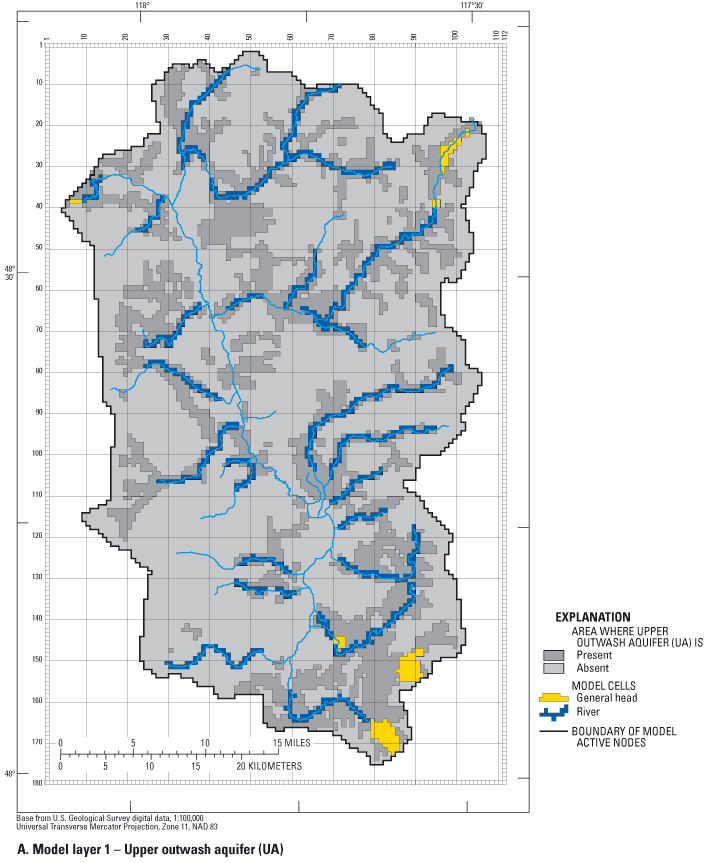
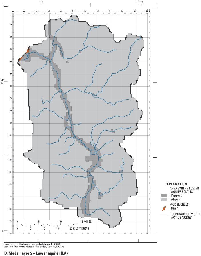
The large cell size and uniform grid spacing were chosen to reflect the regional scale of this study. The predominant flow direction in the study area is from south to north; therefore the grid is oriented similarly. The extents of active cells in each layer are outlined on figures 7A-E.
Five model layers were used to simulate the saturated unconsolidated sediments that overlie the bedrock and one layer of constant thickness was used to simulate the upper bedrock.
| Hydrogeologic unit | Model layer |
|---|---|
| Upper outwash aquifer (UA) | 1 |
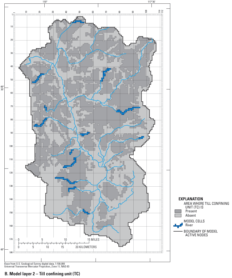
| Till confining unit (TC) | 2 |
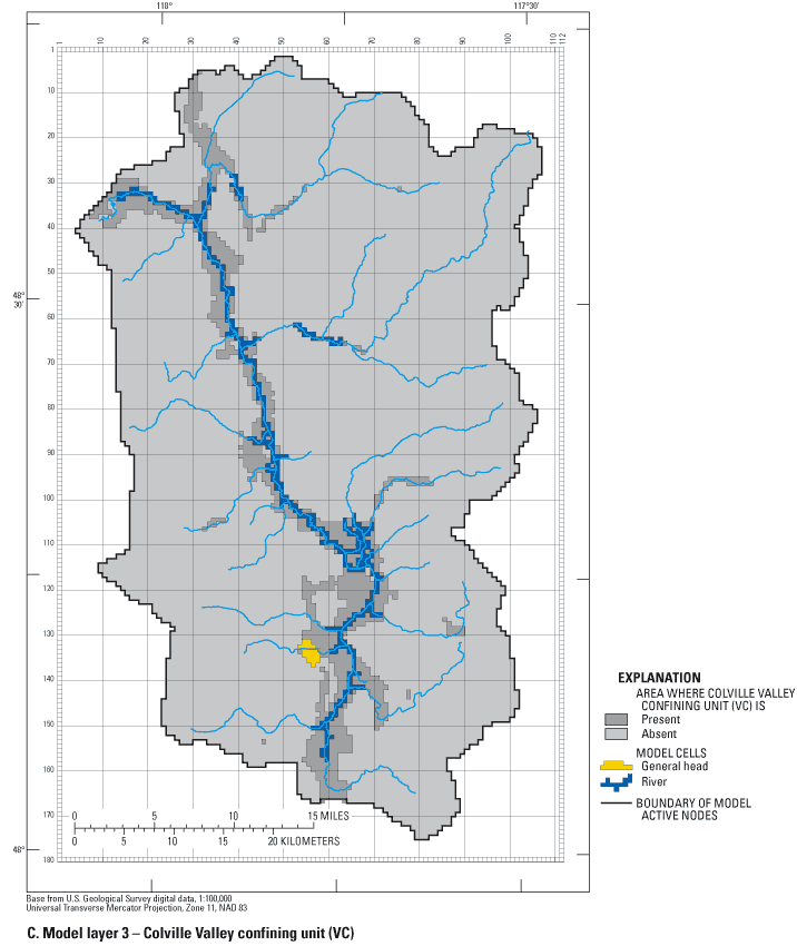
| Colville Valley confining unit (VC) | 3 and 4 |
| Lower aquifer (LA) | 5 |
| Bedrock (BR) | 6 |
All layers were simulated as confined due to numerical instabilities that would occur in the model where relatively thin unsaturated thicknesses could not be accurately simulated because of the coarse model grid. Adjustments were made to unit UA to account for large unsaturated thicknesses in some locations. The adjustments were accomplished by lowering the top of unit UA to correspond with the water table.
The Colville Valley confining unit is present throughout the length of the valley and therefore plays an important role in ground-water/surface-water interaction with the Colville River. MODFLOW represents the exchange of water between the stream and the ground-water system as a function of stream geometry and the difference between the head in the stream and the head at the center of an adjacent underlying model cell. To eliminate errors produced by this representation, the thick Colville Valley confining unit was subdivided into two model layers. Layer 3 is the upper 20 ft of unit VC and the remainder of the unit is layer 4.
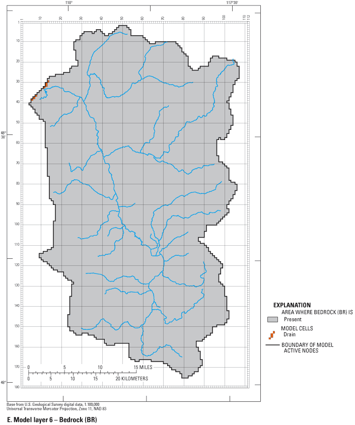
Bedrock has low permeability except for where it is fractured, but the fractures are at too small a scale to be represented in a regional model, and little is known about the hydraulic properties of the bedrock at depth. Owing to these uncertainties and necessary simplifications, layer 6 was assigned a constant thickness of 200 ft.
The MODFLOW-2000 user interface requires that all layers be present in all active nodes in the model. A method similar to one described in Drost and others (1999) was used to ensure proper model operation. A 0.1-foot thickness was assigned where a unit was not present and the hydraulic properties were altered to represent a large vertical hydraulic conductivity (1,000 ft/d) and a small horizontal hydraulic conductivity (0.00001 ft/d). This results in the simulated flow passing vertically through the "missing" layer as if it were not present, while introducing insignificant inaccuracies in lateral flow.
Hydrogeologic Framework
The 3-dimensional digital hydrogeologic framework developed for the ground-water-flow model is based on the primary data used by Kahle and others (2003): Digital Elevation Model (DEM), geologic maps, cross sections, and lithologic well logs. These data types were manipulated with stratigraphic analysis software and a Geographic Information System (GIS).
The electronic data were assembled into one 3-dimensional, spatially distributed hydrogeologic representation using GIS for incorporation into the ground-water-flow model. Existing data included (1) surficial geology maps, (2) map extents of the four unconsolidated hydrogeologic units, (3) well-log point values for tops and thicknesses of units UA, VC, and LA, (4) well-log point values for the top of bedrock, (5) thickness contours for units UA and VC, and (6) 26 hydrogeologic cross sections.
Elevations of each hydrogeologic unit were determined relative to the surface elevation grid (30-meter DEM). A systematic approach was developed using GIS to determine the presence of a unit and, if present, the thickness of that unit. This method was performed at 100-meter resolution and then scaled up to match the model grid. Thickness contours for units UA and VC were converted to values for each cell and subtracted from land surface, if present at the surface, or the bottom of the overlying unit. TC thickness was estimated to range from 10 to 100 ft; little comprehensive thickness data exist. For the ground-water model, an average thickness of 75 ft was assigned where unit TC was present. Thickness data generally are unavailable for unit LA because few wells penetrate the full thickness of the unit. A constant thickness of 200 ft was assigned where LA was present at the surface. In most locations, LA was present beneath unit VC and was assigned a thickness of 75 ft. Bedrock is present at all locations.
The six-layer, 3-dimensional grid was then compared to the 26 hydrogeologic cross sections and adjusted where appropriate. An effort was made to honor the geologist's interpretation so the model construction was as representative as possible. Large data gaps and the regional scale of the ground-water model created some discrepancies, but the method described above created a reproducible hydrogeologic representation that was used to create the model framework.
Boundary Conditions
Boundary conditions in a ground-water-flow model define the locations and manner in which water enters and exits the active model domain. The general conceptual model for the Colville River Watershed is that water enters the system as precipitation and exits the system as streamflow and ground-water discharge near the mouth of the watershed. Three types of boundaries were used in the Colville River Watershed model: no-flow (outer model boundary), head-dependent flux (rivers, drains, and general head) (figs. 7A-E), and specified-flux (recharge). The boundaries of the model coincide as much as possible with natural topographic, geologic, and hydrologic boundaries.
Topographic Boundaries
Major topographic divides primarily define the lateral model boundaries. These natural features act as no-flow boundaries as they are considered coincident with ground-water divides. The topographic divides are either exposed bedrock or bedrock covered by a shallow layer of unconsolidated sediments. The entire outer model boundary is simulated as a no-flow boundary, with the exception of the mouth of the system near Kettle Falls. Water exits the system at this location through both surface-water and ground-water flow. A small section of the southern boundary, near the town of Springdale, probably forms a very shallow ground-water divide. This section is the southern extent of the VC and LA units as mapped within the Colville River Watershed. A stress on the system, such as increased ground-water pumping near the boundary, could induce flow across the boundary.
Hydrologic-Process Boundaries
River Conductances and Stages
Ground-water/surface-water exchange is an important process in the ground-water-flow system and the model. The movement of water between the two systems is controlled by the differences in ground-water hydraulic head and river stage (altitude). The Colville River and 20 tributaries were simulated using the MODFLOW River (RIV) package (figs. 7A-C). Stream stages, which were specified in the model, were determined from USGS 1:24,000 scale topographic maps at stream confluences, streamflow-measurement locations, reaches with steep gradients, and various locations along the streams. Stages were linearly interpolated between input points. Contour intervals on the topographic maps were predominantly 40-foot with a few at 20-foot contour intervals. Stream stages estimated from the maps had an accuracy of plus-or-minus one-half the contour interval. Some inaccuracy was introduced by averaging stream stages and ground-water altitudes within model cells. This uncertainty was not deemed a problem along the gentle relief of the Colville River valley floor but introduced greater uncertainty in the steep headwaters.
The simulated quantity of water moving between the ground-water and surface-water systems is equal to the product of streambed conductance and the head difference between the stream and underlying hydrogeologic units. Streambed conductance was determined empirically during model calibration. Initial values of streambed conductance were based on measured stream width during September 2001, stream length (determined using GIS), and assumed stream depth of 2 ft and streambed thickness of 1 ft for all stream reaches. Initial streambed hydraulic conductivity was assumed to equal the vertical hydraulic conductivity of the hydrogeologic unit in which the stream was in direct connection. Streambed conductances were initially grouped into five parameter values (table 2), as a function of vertical hydraulic conductivity, stream width, and streambed thickness. The values in table 2 reflect all of the terms for streambed counductance except for stream reach length. The model internally mulitplies the value in table 2 (ft/d) by the stream reach length (ft), resulting in the streambed conductance (ft2/d).
Drain Conductances and Stages
The MODFLOW Drain (DRN) package was used to simulate subsurface discharge from the Lower aquifer and Bedrock units below Kettle Falls into Franklin D. Roosevelt Lake. The simulated quantity of water exiting the system at a drain cell is equal to the product of a user-specified drain conductance and the difference between the simulated hydraulic head in the drain cell and the specified altitude of the drain (lake stage). The drain conductance is a function of the surrounding hydrogeologic material and the cell geometry.
The Colville River Watershed model simulates ground water exiting the system at only one location, through the Lower aquifer and Bedrock units below Kettle Falls (figs. 7D-E). All drain altitudes were assigned the stage of Franklin D. Roosevelt Lake in September 2001. The conductances for the drains in the model were computed in the same general way as were the stream conductances, but the assumptions followed those made by Morgan and Jones (1999): the area of the ground-water flow spans the entire width and length of the cell, Hydraulic conductivity was the same as that of the hydrogeologic unit of the cell, and the length of the flowpath was the distance from the cell center to the cell face (750 ft).
[Values for streambed conductance are shown in feet per day and must be multiplied by stream reach length (feet). ft/d, foot per day; in/yr, inch per year]
| Hydrogeologic unit | Parameter label | Value |
|---|---|---|
| Horizontal hydraulic conductivity (ft/d) | ||
| Upper outwash aquifer (UA) | HK_UA | 50 |
| Till confining unit (TC) | HK_TC | 1 |
| Colville Valley confining unit (VC) | HK_VC | 1 |
| Lower aquifer (LA) | HK_LA | 50 |
| Bedrock (BR) | HK_BR | .1 |
| Vertical anisotropy | ||
| Upper outwash aquifer (UA) | VANI_UA | 10 |
| Till confining unit (TC) | VANI_TC | 1,000 |
| Colville Valley confining unit (VC) | VANI_VC | 1,000 |
| Lower aquifer (LA) | VANI_LA | 10 |
| Bedrock (BR) | VANI_BR | 100 |
| Streambed conductance for tributary reaches (ft2/d) | ||
| Colville River | RIV_CLV | 0.034 |
| High—over unit UA | RIV_UA1 | 50 |
| Low—over unit UA | RIV_UA2 | 5 |
| Over unit TC | RIV_TC | .002 |
| Over unit VC | RIV_VC | .007 |
| Area of recharge (in/yr) | ||
| Valley floor | RCH_VAL | 0.5 |
| Low | RCH_LOW | .5 |
| Medium | RCH_MED | 3 |
| High | RCH_HI | 6 |
Lake Conductances and Stages
The MODFLOW general head boundary (GHB) package was used to simulate subsurface discharge from the lakes to the underlying aquifers (figs. 7A and 7C). An external source (lake stage) provides flow into and out of a cell in proportion to the difference between the head in the cell and the specified head of the external source. The specified lake stages were determined from USGS 1:24,000-scale topographic maps with the exception of Loon Lake, where lake stage data were available. The lake-bottom conductance is a function of the surrounding hydrogeologic material and the lake area.
Ground-Water Pumping Rates
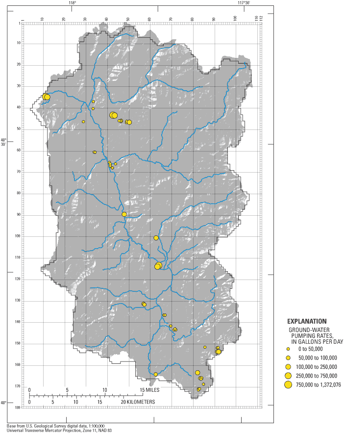
Ground-water pumping rates were specified in the model by two different methods representing public-supply and exempt (domestic) wells. Pumping rates for public-supply wells for September 2001 were derived from reported and estimated water-use data. Forty-five public-supply wells withdrawing a total of 6.0 Mgal/d, or 18.4 acre-ft/d) were assigned to the appropriate location and hydrogeologic unit (table 3; fig. 8).
| Well or system name | Pumping rate(gallons per day) |
|---|---|
| Upper outwash aquifer (UA) | |
| Arden Hills Water System | 12,474 |
| Chewelah Golf Course, City of | 121,567 |
| Colville, City of | |
| S01 | 56,900 |
| S03 | 0 |
| S02 | 17,733 |
| S04 | 522,167 |
| S06 | 103,267 |
| S07 | 941,433 |
| Country Villa Mobile Park | 594 |
| Crossroads Café | 480 |
| Dominion View Water Association | 10,692 |
| Elm Tree Water and Sewer Association | 8,316 |
| Granite Point Park | 594 |
| Kettle Falls (well 4) | 457,292 |
| Pine Grove Menonite Church | 87 |
| Pinelow Park | 4,376 |
| Springdale, City of | 85,536 |
| Stevens County | |
| PUD—Deer Lake, S03 | 135,269 |
| PUD—Loon Lake SW, S01 | 23,964 |
| PUD—Loon Lake SW, S02 | 34,090 |
| PUD—Jump off Joe Lake | 38,642 |
| PUD—Jump off Joe Lake | 3,973 |
| PUD—Loon Lake shop, S01 | 221,313 |
| PUD—Valley, S01 | 20,340 |
| PUD—Valley, S02 | 0 |
| PUD—Sunset Bay, S03 | 34,122 |
| PUD—Sunset Bay New, S04 | 77,114 |
| Colville Valley confining unit (TC) | |
| Stevens County | |
| PUD—Waitts Lake, S01 | 52,237 |
| PUD—Waitts Lake, S02 | 60,400 |
| Stimson (domestic use) | 4,800 |
| Lower aquifer (LA) | |
| Chewelah, City of | |
| S03 | 299,500 |
| S04 | 763,933 |
| Kettle Falls (wells 2, 3, and 5) | 1,371,875 |
| NW Alloys (well field) | 175,667 |
| Panorama Mobile Home Park | 297 |
| Stevens County PUD (Jump off Joe Lake) | 3,973 |
| Bedrock (BR) | |
| Corbett Creek Water System | 23,760 |
| Panorama Mobile Home Park | 297 |
| Stevens County | |
| PUD—Deer Lake, S03 | 135,269 |
| PUD—Loon Lake SW, S01 | 23,964 |
| PUD—Sunset Bay New, S04 | 77,114 |
| Timothy Park Subdivision (3 wells) | 2,376 |
| Town of Addy Stevens County | |
| PUD—S02 | 22,161 |
| PUD—S03 | 40,579 |
| Williams Lake Road Subdivision | 8,316 |
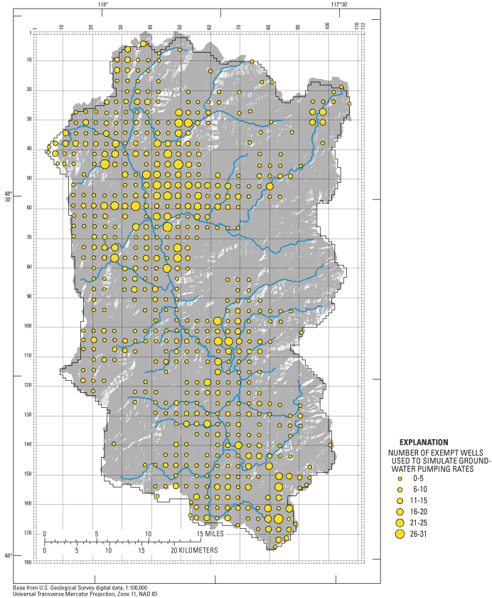
Less information is available for exempt wells. The DOE maintains a database of exempt wells located only by township, range, section, and quarter section, resulting in more than one well at most model cells (fig. 9). No information existed as to which hydrogeologic units the wells were open. The DOE database contained 3,600 wells at 569 locations. (All wells in the DOE database are not active and some wells that are not in the database existed before the DOE began keeping records.) Pumping rates were calculated by dividing the total estimated ground-water pumpage from exempt wells (1.7 Mgal/d) (Kahle and others, 2003) by the total number of exempt wells. Simulated annual pumpage was 472 gal/d per exempt well. The pumping rate was then multiplied by the number of wells assigned to each pumping cell. The well was assigned to a model layer on the basis of a simple assumption. If the Upper aquifer existed at the well location, the well was assigned to model layer 1. If no UA existed and LA did exist, the well was assigned to model layer 5. If neither UA nor LA existed at the location, the well was assigned to model layer 6 (Bedrock). Because the well location was approximate, this assumption probably resulted in the assignment of too few wells to model layer 1 and too many wells to model layer 6.
Simulated pumpage from exempt wells accounted for only 6.5 percent of total ground-water use. The approximations involved in estimating the exempt wells were considered sufficient because of the relatively small percentage of the total ground-water budget they represent.
Recharge
The Precipitation-Runoff Modeling System (PRMS) (Leavesley and others, 1983) was used to compute initial ground-water recharge estimates. Kahle and others (2003) provided long-term average annual ground-water recharge estimates for the entire watershed, but the ground-water-flow model requires spatially distributed recharge for the simulation period.
In PRMS, a watershed is conceptualized as an interconnected series of reservoirs whose collective output produces the total hydrologic response. These reservoirs include interception storage in the vegetation canopy, storage in the soil zone, subsurface storage between the surface of a watershed and the water table, and ground-water storage. The system inputs included daily precipitation and daily maximum and minimum air temperature. Streamflow at a watershed outlet is the sum of surface, subsurface, and ground-water flows.
Surface runoff is related to a dynamic source area that expands and contracts to precipitation characteristics, and to the capability of the soil mantle to store and transmit water (Troendle, 1985). As conditions become wetter, the proportion of precipitation diverted to surface runoff increases, while the portion that infiltrates to the soil zone and subsurface reservoirs decreases. Daily infiltration is computed as the net precipitation minus surface runoff. Precipitation retained on the land surface is modeled as surface-retention storage. Once the maximum retention storage is satisfied, excess water becomes surface runoff. When free of snow, the retention storage is depleted by evaporation.
Precipitation that falls through the vegetation canopy infiltrates the soil zone. The soil zone is conceptualized as a two-layer system. Moisture in the upper soil (or recharge) zone and in the lower soil zone is depleted through root uptake and seepage to lower zones. Evaporation also depletes the upper soil zone of moisture. The depths of the soil zones are defined on the basis of water-storage characteristics and the average rooting depth of the dominant vegetation.
Potential evapotranspiration (PET) losses were computed as a function of solar radiation and the number of cloudless days (Jensen and Haise, 1963). When soil moisture is available, evapotranspiration equals PET. When soil moisture is limiting, actual evapotranspiration (AET) is computed from PET-to-AET relations for soil types as a function of the ratio of current available water in the soil profile to the maximum available water holding capacity of the soil profile (Zahner, 1967).
Water can move to a ground-water reservoir from both the soil zone and the subsurface reservoir. Soil water in excess of field capacity moves to the ground-water reservoir and is limited by a maximum daily recharge rate. When average moisture exceeds this daily rate, excess soil water moves to the subsurface reservoir. Excess moisture in the subsurface reservoir either percolates to a ground-water reservoir or flows to a discharge point above the water table. Seepage to the ground-water reservoir is computed first from the soil zone and then as a function of a recharge rate coefficient and the volume of water in the subsurface reservoir. The ground-water reservoir is the source of all baseflow and water entering this reservoir is considered recharge.
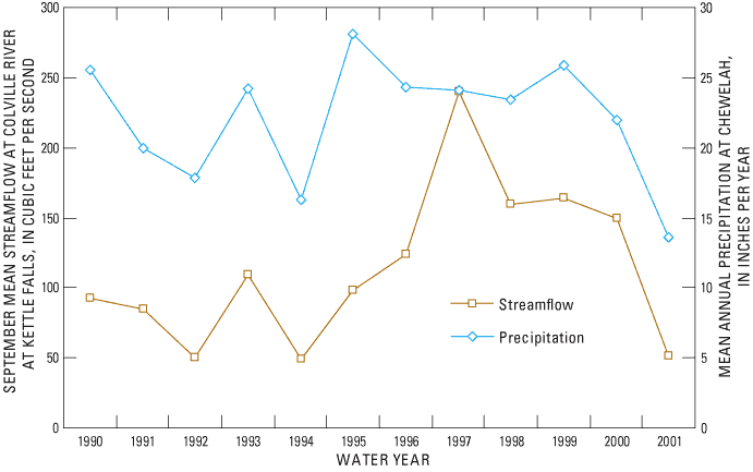
Most snow, and thus spring runoff from snowmelt, originates at high altitudes. Annual snowpack is depleted by mid-July. The simulation period, September 2001, was the low-flow period of a low precipitation year. Mean annual streamflow for the Colville River at Kettle Falls for 1923-2001 is 309 ft3/s, and September mean streamflow is 97.5 ft3/s. The September 2001 monthly mean streamflow was only 50.9 ft3/s. The simulation period does not represent either a mean annual value or a mean September value.
An evaluation of mean annual precipitation at Chewelah, and September mean flow of the Colville River (fig. 10) shows contribution from precipitation to recharge occurs on an annual basis. During late summer and autumn, ground-water discharge contributes a substantial portion of baseflow. Water year 2001 (October 2000 – September 2001) was an extremely low precipitation year and baseflow for that time period also was extremely low. This relation demonstrates that most precipitation recharged to the ground-water system is discharged to the surface-water system within an annual cycle.
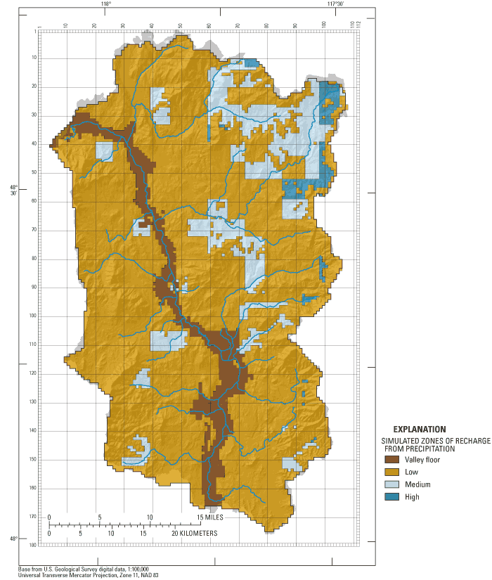
Simulated (model) recharge from precipitation was determined from the initial mean annual recharge estimates from PRMS. Estimated recharge from PRMS reflects the net effect of precipitation, surface runoff, evapotranspiration, and water released from storage and can be considered an "effective" recharge rate (Halford, 1999). The simulated recharge was then lumped into four recharge zones – valley floor, low, medium, and high (table 2; fig. 11). Precipitation generally is lowest at the low altitudes along the main valley floor. Additionally, the valley floor has the low-permeability valley confining unit at the surface. Recharge along the valley floor was initially assigned a value of 0.5 in/yr. Most snowpack resides in the high altitudes on exposed bedrock, a unit with very low infiltration rates. To represent the depleted snowpack and minimal recharge through the bedrock, all recharge simulated where bedrock was exposed at the surface was uniformly reduced to 0.5 in/yr, the rate for the low recharge zone. This procedure "removed" much of the snow from the simulation in order to represent baseflow conditions. The recharge rate for the medium recharge zone was specified at 3 in/yr and the recharge rate for the high recharge zone was specified at 6 in/yr.
Secondary recharge was simulated by hypothetical injection wells. In most instances, secondary recharge was applied to the row and column in the model grid from which water was withdrawn (pumped) but assigned to the uppermost model layer to reflect the shallow nature of septic systems relative to ground-water pumping. If the location of the public sewage disposal facility was known, that location was assigned as a secondary recharge point. A uniform rate of 50 percent of ground-water pumping was applied for secondary recharge.
Recharge from irrigation was assumed equivalent to deep percolation. Seventy-five model cells representing areas of irrigation were assigned a uniform recharge rate of 4.3 in/yr, which is 12 percent of a 36 in/yr application rate (Drost and others, 1997), totaling 2.5 Mgal/d. The presumed application rate is an average water requirement for alfalfa (Molenaar and others, 1952; James and others, 1982; Cline and Collins, 1992; Ely, 2003). The location of irrigated agricultural areas was determined from the USGS National Land Cover Data map.
Model Flow Parameters
Initial Horizontal Hydraulic Conductivity
Horizontal hydraulic conductivities used for the hydrogeologic units in the model were those determined from specific-capacity data (Kahle and others, 2003). The scarcity and lack of trends in the existing data precluded an initial zonation of hydraulic conductivity. Because there is no evidence that hydraulic conductivity varies with direction, horizontal isotropy was assumed, and each model layer was assigned one horizontal hydraulic conductivity (table 2). An initial value of 50 ft/d was used for hydrogeologic units UA and LA. The confining units were assumed to have horizontal hydraulic conductivities of 1 ft/d. Bedrock hydraulic conductivity was uniformly specified at 0.1 ft/d.
Initial Vertical Hydraulic Conductivity
Vertical hydraulic conductivities were initially derived as ratios of the vertical to the horizontal values (table 2). The ratios for aquifers were assumed to be 1:10, and for confining units, were initially assumed to be 1:1,000. Bedrock ratios were assumed to be 1:100.
Model Calibration
The steady-state Colville River Watershed ground-water-flow model was calibrated to September 2001 conditions. September 2001 does not represent average conditions, as it was an extremely dry period. Therefore, all results and alternatives derived from the model simulations are a conservative representation of the system. The below-average precipitation during water year 2001 would cause a decline in water levels, but whether that decline was fully observed by September 2001, when water levels were measured, is unknown. Differences between water levels measured in late summer 2001 and spring 2002 are small relative to the overall, long-term range in water levels and the large hydraulic gradients present in the tributary basins, and would be within the range of model error. The primary reason for choosing the September 2001 conditions for calibration is the existence of basin-wide synoptic water-level and streamflow measurements for this period. Streamflow measurements provide the best calibration targets and most effectively constrain the calibration process. Long-term water-level data are scarce but nothing in the record suggests that the regional ground-water-flow system in the Colville River Watershed is not in long-term equilibrium with the natural climatic cycle.
The calibration procedure used in this study largely followed that used and described by Gannett and Lite (2004) for their study in the Upper Deschutes River Watershed, Oregon. The theory behind the method of nonlinear regression and automated calibration follow the techniques described by Cooley and Naff (1990). Hill (1998) presents the methods and guidelines for effective model calibration.
Calibration Data
The hydraulic-head data used for calibration consisted primarily of water-level measurements in 161 wells between August and November 2001. An attempt was made to acquire a uniform areal distribution of water-level measurements in wells completed in the unconsolidated deposits of the study area, including the main Colville River valley floor and side valleys. This was not possible in all areas, however, mostly due to lack of development in much of the watershed and to a much lesser extent, lack of access to wells (Kahle and others, 2003). Depth to water (water level) was measured in most wells using a calibrated electric tape or graduated steel tape, both with accuracy to 0.01 ft. Well locations were plotted on USGS 1:24,000-scale topographic maps. Altitude of the land surface at each site was interpolated from the topographic maps, with an accuracy of ±20 ft (one-half the contour interval). A Global Positioning System (GPS) receiver with a horizontal accuracy of one-half a second (about 50 ft) was used to determine latitude and longitude at each well. Water-level measurements in wells completed in bedrock were not used in the calibration. Information from the bedrock wells was used, however, to help understand the connection between the unconsolidated deposits and the bedrock unit.
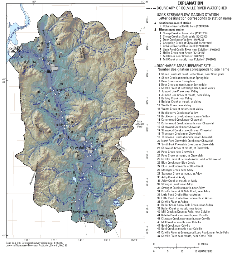
Synoptic streamflow measurements were made along the Colville River and its tributaries to quantify the ground-water discharge to, or recharge from, the surface-water system at baseflow conditions, and to identify gaining and losing reaches of the stream over the unconsolidated valley deposits. To identify gaining and losing stream reaches, a low-flow seepage run (a set of streamflow measurements representing approximately steady-flow conditions) was conducted in early September 2001 with a few follow-up measurements in early October 2001. The September time frame was chosen because streamflows in the watershed are usually near their annual minimums at this time, and fluctuation owing to precipitation also is minimal, allowing for meaningful comparison of measurements. Calibration of this model benefited greatly from the availability of these streamflow measurements. A total of 78 streamflow measurements plus 3 observations of no flow were made during the study (table 4; Kahle and others 2003). Some of these measurements were made at active or discontinued streamflow-gaging stations, but most were made at sites that had not been previously measured (fig. 12).
[ft3/s, cubic foot per second; oC, degrees Celsius; –, no data]
| Map No. (see fig. 12) |
Site name | Date | Discharge (ft3/s) |
Water temperature(oC) |
|---|---|---|---|---|
| B | Sheep Creek at Springdale (station 12407500) | 09-04-01 | 5.55 | – |
| 04-16-02 | 10.9 | 6.5 | ||
| 1 | Sheep Creek at Forest Center Road, near Springdale | 09-04-01 | 8.02 | 16.5 |
| 04-16-02 | 11.9 | 9 | ||
| 2 | Sheep Creek at mouth, near Springdale | 09-11-01 | 6.91 | 14.5 |
| 3 | Deer Creek near Springdale | 09-05-01 | 4.66 | 11 |
| 04-23-02 | 63.5 | 5.5 | ||
| 4 | Deer Creek at mouth, near Springdale | 09-11-01 | 4.13 | 13 |
| 5 | Colville River at Betteridge Road, near Valley | 09-05-01 | 12.9 | 15 |
| 04-17-02 | 163 | 5.5 | ||
| 6 | Jumpoff Joe Creek near Valley | 09-05-01 | 2.77 | 15.5 |
| 04-11-02 | 7.97 | 9.5 | ||
| 04-16-02 | 9.92 | 10 | ||
| 7 | Jumpoff Joe Creek at mouth, near Valley | 09-11-01 | 2.75 | 18.5 |
| 8 | Bulldog Creek near Valley | 09-11-01 | 2.84 | 10 |
| 04-11-02 | 4 | 9 | ||
| 08-16-02 | 4.62 | 11 | ||
| 9 | Bulldog Creek at mouth, at Valley | 10-02-01 | 1 7.32 | – |
| 08-16-02 | 1 7.97 | 13.5 | ||
| 10 | Waitts Creek near Valley | 10-02-01 | .11 | – |
| 11 | Waitts Creek at mouth, near Valley | 10-02-01 | .18 | – |
| 12 | Huckleberry Creek near Valley | 09-05-01 | .52 | 13.5 |
| 04-18-02 | 106 | 5 | ||
| 13 | Huckleberry Creek at mouth, near Valley | 09-11-01 | .07 | 18 |
| 14 | Cottonwood Creek near Chewelah | 09-05-01 | 2.38 | 17.5 |
| 04-12-02 | 46.4 | 7.5 | ||
| 15 | Cottonwood Creek at mouth, near Chewelah | 09-11-01 | 2.71 | 18 |
| 16 | Sherwood Creek near Chewelah | 09-05-01 | .52 | 13.5 |
| 04-15-02 | 12 | 4.5 | ||
| 17 | Sherwood Creek at mouth, near Chewelah | 09-13-01 | .42 | 13 |
| 18 | Thomason Creek near Chewelah | 09-07-01 | .89 | 10.5 |
| 04-15-02 | 1.73 | 4.5 | ||
| 19 | Thomason Creek at mouth, near Chewelah | 09-13-01 | .76 | 12.5 |
| 20 | North Fork Chewelah Creek near Chewelah | 09-07-01 | 3.73 | 10 |
| 04-18-02 | 103 | 5.5 | ||
| 21 | South Fork Chewelah Creek near Chewelah | 09-07-01 | 3.65 | 10 |
| 04-19-02 | 36.6 | 3.5 | ||
| 22 | Chewelah Creek at mouth, at Chewelah | 09-13-01 | 7.14 | – |
| 23 | Paye Creek near Chewelah | 09-07-01 | 3.39 | 11 |
| 04-15-02 | 4.37 | 5.5 | ||
| 24 | Paye Creek at mouth, at Chewelah | 09-13-01 | 3 | – |
| 25 | Colville River at Schmidlekofer Road, at Chewelah | 09-11-01 | 31.6 | 14 |
| 04-17-02 | 757 | 9 | ||
| 26 | Blue Creek near Blue Creek | 09-06-01 | .09 | 10 |
| 04-15-02 | 2.88 | 7 | ||
| 27 | Blue Creek at mouth, at Blue Creek | 09-13-01 | 0.04 | – |
| E | Colville River at Blue Creek (station 12408000) | 09-05-01 | 31.3 | 17 |
| 04-17-02 | 707 | 9 | ||
| 28 | Stensgar Creek near Addy | 09-06-01 | .32 | 14 |
| 04-15-02 | 90.2 | 5.5 | ||
| 29 | Stensgar Creek at mouth, at Addy | 09-13-01 | .04 | – |
| 30 | Addy Creek at Addy | 09-06-01 | .1 | 12 |
| 04-16-02 | 11.8 | 4 | ||
| 31 | Addy Creek at mouth, at Addy | 09-13-01 | .01 | – |
| 32 | Stranger Creek near Addy | 09-06-01 | .24 | 14 |
| 04-16-02 | 62.1 | 5 | ||
| 33 | Stranger Creek at mouth, near Addy | 09-13-01 | .04 | – |
| 34 | Colville River at 12 Mile Road, near Addy | 09-06-01 | 30.9 | 15 |
| 04-15-02 | 753 | 8.5 | ||
| 35 | Little Pend Oreille River at Arden | 09-05-01 | 13.6 | 15 |
| 04-24-02 | 290 | 4 | ||
| 36 | Little Pend Oreille River at mouth, at Arden | 09-13-01 | 9.63 | – |
| 37 | Colville River at Arden | 09-05-01 | 40.6 | 16 |
| 04-17-02 | 1,040 | 7.5 | ||
| 38 | Haller Creek below Cole Creek, near Arden | 09-06-01 | .96 | 8 |
| 04-12-02 | 22.3 | 5 | ||
| 39 | Haller Creek at mouth, near Arden | 09-13-01 | no flow | – |
| H | Mill Creek near Colville (station 12408500) | 09-04-01 | 4.73 | 13 |
| 04-24-02 | 171 | 3 | ||
| 40 | Mill Creek at Douglas Falls, near Colville | 09-04-01 | 3.77 | 12 |
| 04-24-02 | 197 | 5.5 | ||
| 41 | Gillette Creek near mouth, near Colville | 08-27-01 | no flow | – |
| 42 | Clugston Creek near mouth, near Colville | 09-07-01 | .38 | 14 |
| 04-19-02 | 3.95 | 4 | ||
| 43 | Mill Creek at mouth, near Colville | 09-13-01 | 6.41 | 19 |
| 44 | Gold Creek near Colville | 09-07-01 | .003 | 14 |
| 04-16-02 | 22.2 | 5 | ||
| 45 | Gold Creek at mouth, near Colville | 08-27-01 | no flow | – |
| 46 | Colville River at Greenwood Loop Road, near Kettle Falls | 09-04-01 | 2 46.7 | 18 |
| 04-15-02 | 1,630 | 6.5 | ||
| J | Colville River at Kettle Falls (station 12409000) | 09-04-01 | 46 | – |
| 04-15-02 | 2 1,560 | – | ||
| 08-16-02 | 3 61 | 21 | ||
| 47 | Colville River near mouth, near Kettle Falls | 08-16-02 | 59.4 | 23 |
| 1 Includes 0.67 ft3/s discharge from Lane Mountain Silica Plant. | ||||
| 2 Daily mean discharge. | ||||
| 3 Instantaneous discharge at time discharge was measured at Colville River near mouth, near Kettle Falls on August 16, 2002. | ||||
(From Kahle and others, 2003.)
Steady-State Calibration Procedure
The steady-state calibration procedure was done using MODFLOW-2000's Observation, Sensitivity, Parameter Estimation (OSP) process (Hill and others, 2000). The OSP process uses a nonlinear least-squares regression to find the set of parameter values that will minimize the weighted sum-of-squared-errors objective function (Hill, 1998):
![]() , (1)
, (1)
| where | |
|
|
is a vector containing values for each of the parameters being estimated, |
|
|
is the number of observations, |
|
|
is the ith observation being matched by regression, |
|
|
is the simulated value corresponding to the ith observation, and |
|
|
is the weight assigned to the ith observation. |
The differences between the measured and simulated values are residuals. Residuals are weighted to allow a meaningful comparison of measurements with different units (weighted residuals are dimensionless) and to reduce the influence of measurements with large errors or uncertainty. The observation weight is defined as the inverse of the variance of the measurement error.
The observation weights were assigned using the methods suggested by Hill (1998). Hydraulic-head measurement errors were limited by the accuracy of the topographic map used to determine land-surface altitude. As previously noted, the depth to water measured by a calibrated electric tape or graduated steel tape was accurate to 0.01 ft. That measurement, however, was then subtracted from a land-surface altitude with an accuracy of ±20 ft. A standard deviation of measurement error was estimated for each measurement by assuming that the 95-percent confidence interval for the actual head was equal to the hydraulic-head measurement ± 0.5 the contour interval of the topographic map used to determine the well altitude.
Discharge measurements used to calibrate the Colville River Watershed model also were weighted by estimating the standard deviation of the measurement error. The USGS rates the accuracy of its streamflow records based on the quality of the measurements. Accuracy levels of "good" indicate that 95 percent of the measurements are within 10 percent of the actual values and "fair" indicates that 95 percent of the measurements are within 15 percent of actual values. On the basis of field notes supplied by the hydrologic technicians that completed the measurements, all measurements were "good." Where a single discharge measurement was used as a flow observation in the model, the confidence interval was ±10 percent. Where the observation was the gain or loss between two discharge measurements, the combined error of both measurements defined the confidence interval.
Model Parameters
Hill (1998) discusses the importance of parsimony in model construction. Building a complex model with more parameters than the data support may reduce the residuals but does not ensure a more accurate, reliable model. Following the principle of parsimony, only selected hydraulic parameters and stresses were estimated during calibration. The drain conductances near Kettle Falls, lake conductances, and ground-water pumping rates were not adjusted during calibration. No data exist to estimate ground-water flow out of the system or recharge from lakebed seepage. Ground-water pumping rates were supplied by the Planning Team and were considered reliable. The parameters adjusted during calibration included horizontal hydraulic conductivities, recharge zones, and river conductances. Throughout the calibration process, no adjustments were made that conflicted with the general understanding of the geology and hydrology.
Parameter Sensitivity
The ability to estimate a parameter value using nonlinear regression is a function of the sensitivity of simulated values to changes in the parameter value. Parameter sensitivity reflects the amount of information about a parameter provided by the observation data. Generally speaking, if a parameter has a high sensitivity, observation data exist to effectively estimate the value. If the parameter has low sensitivity, changing the parameter value will have little effect on the sum of squared errors.
The diagnostic statistics generated by MODFLOW-2000 were the dimensionless scaled sensitivities and the composite scaled sensitivities (Hill, 1998). Dimensionless scaled sensitivities indicate the sensitivity of the simulated equivalent of each observation (here, hydraulic heads and streamflow) to the parameter. The dimensionless scaled sensitivity, ssij, is calculated as (Hill, 1998):
![]() , (2)
, (2)
| where | |
|
|
identifies one of the observations, |
|
|
identifies one of the parameters, |
|
|
is the simulated value associated with the ith observation, |
|
|
is the jth estimated parameter, |
|
|
is the sensitivity of the simulated value associated with the ith observation with respect to the jth parameter, and is evaluated at the final parameter values; and |
|
|
is the weight for the ith observation. |
Composite scaled sensitivities (CSS) summarize all the sensitivities for one parameter. CSS are calculated for each parameter using the scaled sensitivities for all observations (here, hydraulic heads and streamflow). Because they are dimensionless, CSS can be used to compare the amount of information provided by different types of parameters. Model simulation results will be more sensitive to parameters with large CSS. The CSS for the jth parameter, cssj, is calculated as (Hill, 1998):
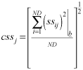 , (3)
, (3)
| where | |
|
|
is the number of observations being used in the regression, |
|
|
is a vector which contains the parameter values at which the sensitivities are evaluated; |
The CSS of all parameters at their initial values divided by the maximum CSS (normalized) are shown in figure 13. Large initial CSS for the hydraulic conductivity of unit UA indicated sufficient information existed to support some zonation of the parameter. Initial hydraulic head and streamflow residuals supported the addition of another zone of hydraulic conductivity. A zone of lower hydraulic conductivity was added to unit UA in the upper reaches of Clugston, Chewelah, and Thomason Creeks.
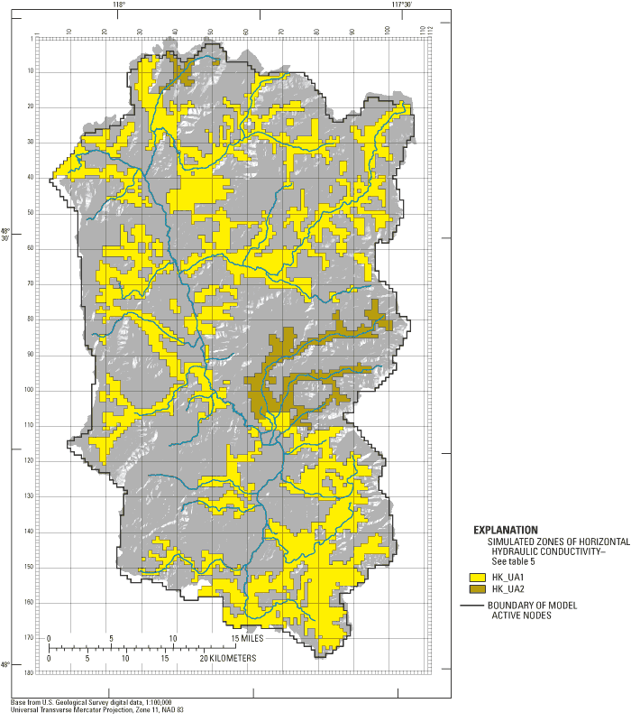
Final Parameter Values
The final parameter values are shown in table 5 and the normalized CSS for all parameters are shown in figure 14. Simulated zones of hydraulic conductivity for model layer 1, Upper outwash aquifer, is shown in figure 15. Hydraulic conductivity for most of unit UA, which represents mostly glacial outwash sand and gravel, was estimated to be 50 ft/d. Simulated hydraulic conductivity for unit TC, which represents compacted and poorly sorted clay, silt, sand, gravel, and cobbles, was estimated to be 0.25 ft/d. Simulated hydraulic conductivity for unit VC, which represents a thick, low-permeability unit consisting mostly of extensive glaciolacustrine silt and clay, was estimated to be 0.25 ft/d. Simulated hydraulic conductivity for unit LA, which represents mostly sand and some gravel, was estimated to be 250 ft/d. This final parameter value for unit LA is higher than the mean value reported in Kahle and others (2003) but falls within the reported range. A difference in depositional mechanisms for units UA and LA could explain the large difference in simulated horizontal hydraulic conductivity. Unit LA perhaps represents a period of major streamflow through the valley and out to the south (prior to the emplacement of the end moraine). Unit UA may have originated from more localized outwash flows. Hydraulic conductivity for bedrock was specified at 0.1 ft/d.
Vertical anisotropy, the ratio of vertical to horizontal hydraulic conductivity, was assigned a value of 1:10 for units UA and LA and 1:1,000 for unit TC. The regression was insensitive to these parameters so no estimation was performed. The vertical anisotropy for unit VC was assigned a value of 1:100. The vertical anisotropy for the bedrock unit was assigned a value of 1:100.
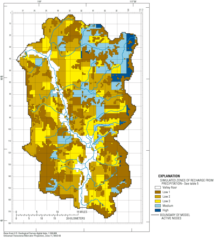
Final recharge rates generally were adjusted downward to match both hydraulic heads and streamflow. Recharge along the Colville River valley floor was estimated to be 0.25 in/yr. Large initial CSS for the "Low" recharge zone supported its subdivision into three recharge zones based on precipitation, elevation, and soil type. Recharge on bedrock (RCH_LOW1) remained 0.5 in/yr. Zone of low recharge 2 (RCH_LOW2) also was 0.5 in/yr. Zone of low recharge 3 (RCH_LOW3) was estimated to be 1 in/yr. The zone of medium recharge (RCH_MED) was adjusted to 2 in/yr. The zone of high recharge (RCH_HI) remained 6 in/yr. Final recharge zones and rates are shown in figure 16 and table 5.
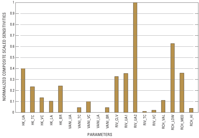
Figure 13. Initial normalized composite scaled sensitivities of model parameters.
Streambed conductances were based on measured stream depth, stream width, and streambed thickness, which was estimated to be 1 ft. Streambed hydraulic conductivity was initially assigned the value of the vertical hydraulic conductivity of the surrounding hydrogeologic unit. During the calibration phase, however, the streams were grouped by the predominant hydrogeologic unit in which they flowed and were adjusted to achieve a good fit between simulated and measured gains and losses. Streambed conductance values of tributary reaches that flowed over unit TC and VC were assigned a value of 0.002 and 0.007 ft/d, respectively, and multiplied by the stream reach length. The greatest streambed conductance was assigned to Sheep Creek (100 ft/d × stream reach length) to reflect the coarse material present along the stream. Streambed conductance values for the Colville River and tributaries that flowed over unit UA were estimated during calibration.
No information exists to constrain drain and lake conductances, and no data exist for ground-water flow out of the model domain. Therefore, the conductances were based on the geometry of the boundary condition and the hydraulic conductivity of the surrounding hydrogeologic unit. No adjustments were made to these parameters.
Steady-State Calibration Model Fit
The measure of model fit can be represented with many statistical and graphical methods, as described by Hill (1998). One measure of model fit is based on the difference between simulated and measured heads and flows, or residuals. The overall magnitude of the residuals is considered, but the distribution of those residuals, both statistically and spatially, can be equally important. The magnitude of residuals can initially point to gross errors in the model, the data (measured quantity), or how the measured quantity is simulated (Hill, 1998). As the model is refined and gross errors are corrected, more complex statistics are examined. Several statistical and graphical analyses of residuals are presented in this section. A complete discussion of the statistical measures discussed in this section is found in Hill (1998).
[The confidence intervals are not symmetric about the estimated value for the log-transformed parameters.Values for streambed conductance are shown in feet per day and must be multiplied by stream reach length (feet). ft/d, foot per day; in/yr, inch per year]
| Hydrogeologic unit | Parameter label |
Estimated value |
95-percent linear confidence upper/ lower intervals on the estimate |
|---|---|---|---|
| Horizontal hydraulic conductivity (ft/d) | |||
| Upper outwash aquifer (high) | HK_UA1 | 50 | 80.9 / 30.9 |
| Upper outwash aquifer (low) | HK_UA2 | 10 | 35 / 2.9 |
| Till confining unit | HK_TC | .25 | 2.03 / 0.03 |
| Colville Valley confining unit | HK_VC | .25 | 94.5 / 0.0007 |
| Lower aquifer | HK_LA | 250 | 431 / 145 |
| Bedrock | HK_BR | .1 | 0.26 / 0.04 |
| Streambed conductance for tributary reaches (ft/d) | |||
| Colville River | RIV_CLV | 0.1 | 0.16 / 0.06 |
| High—over unit UA | RIV_UA1 | 2 | 6.0 / 0.7 |
| Low—over unit UA | RIV_UA2 | 1 | 1.7 / 0.6 |
| Area of recharge (in/yr) | |||
| Valley floor | RCH_VAL | 0.25 | 5.9 / 0.01 |
| Bedrock | RCH_LOW1 | .5 | 1.3 / 0.2 |
| Low–1 | RCH_LOW2 | .5 | 1.0 / 0.2 |
| Low–2 | RCH_LOW3 | 1 | 1.8 / 0.5 |
| Medium | RCH_MED | 2 | 3.4 / 1.2 |
| High | RCH_HI | 6 | 50.8 / 0.7 |
Statistical Measures of Model Fit and Parameter Uncertainty
A commonly used indicator of the overall magnitude of the weighted residual is the calculated error variance. The calculated error variance is the weighted sum of squared errors from equation 1 divided by the number of observations, minus the number of parameters. The square root of the calculated error variance is called the standard error of regression. Smaller values of both terms indicate a closer fit to the measured values. The expected value for both terms is 1.0 if the model fit is completely consistent with the data accuracy, but the calculated error variance is almost always greater than 1.0. The calculated error variance and standard error of regression for the calibrated model in this study are 150.6 and 12.3, respectively.
The calculated error variance and standard error of regression are dimensionless and therefore not intuitively informative about goodness of fit. The fitted standard deviation is the product of the standard error of regression and the statistic used to determine weights. The weights for hydraulic heads in the model are based on the error introduced by determining well altitudes from the topographic maps. For the hydraulic heads alone, the standard error of regression is 8.8. In this study, all hydraulic heads were assigned the standard deviation of measurement error of 10.2 ft. Multiplying this value by the standard error of regression results in a fitted standard deviation for heads of 89.8 ft. The fitted standard deviation represents the overall fit of the hydraulic heads.
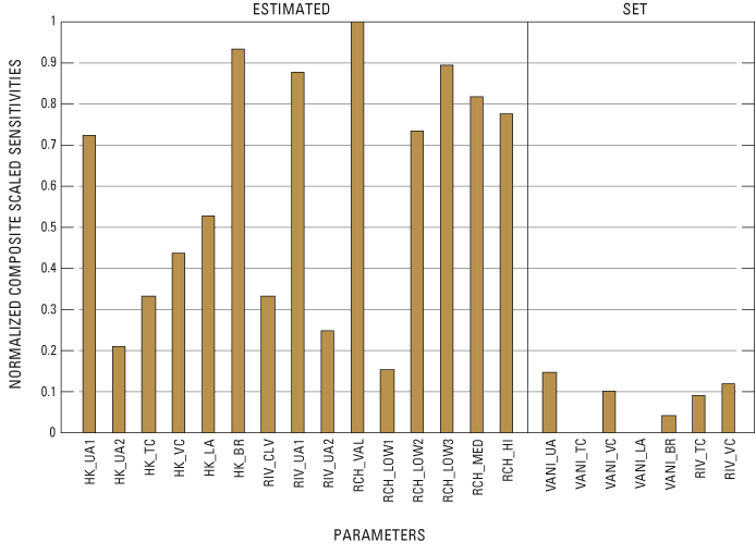
Figure 14. Final normalized composite scaled sensitivities of model parameters.
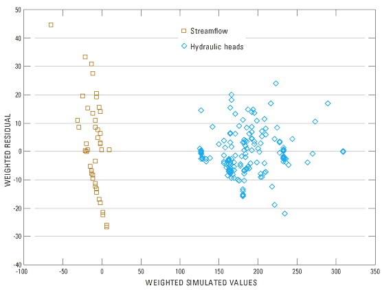
Weighted residuals should be independent, random, and normally distributed. A graphical analysis of the weighted residuals should display an evenly scattered distribution about 0.0. No trends should be apparent, such as consistently larger residuals in a specific hydrogeologic unit or area of the model. Weighted residuals plotted in figure 17 generally meet these conditions for hydraulic heads. The average weighted residual ideally equals zero, and the calibrated model produces an absolute value of the average hydraulic head weighted residual of 0.1. A large bias exists, however, for the streamflow weighted residuals. Of the 44 streamflow measurements, 31 were less than 1.0 ft3/s. The model generally did not reproduce the losing reaches. Most discharge measurements were made along the valley floor, where simulated hydraulic heads generally exceeded measured hydraulic heads. The movement of water between the ground-water and surface-water systems is controlled by the differences in hydraulic head and river altitude. The hydraulic head bias along the valley floor would, therefore, result in a similar bias in simulated discharge. The absolute value of the average weighted residual for all observations was 0.3.
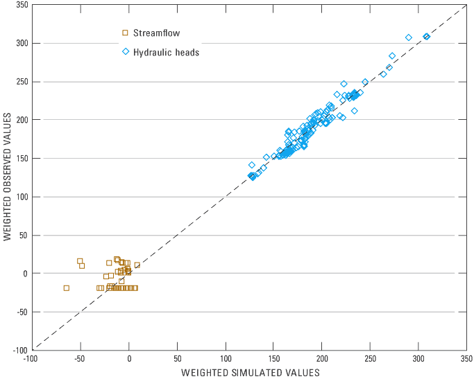
A useful graphical analysis is a simple plot of weighted observations as a function of weighted simulated values. The residuals should plot close to a line with a slope equal to 1.0 and an intercept of zero. The weighted observations versus weighted simulated values shown in figure 18 generally fall along a straight line with a slope of 1.0 but an intercept of 4.4. The significant deviation from the zero intercept is caused by the streamflow residuals.
Another statistic for testing the normality of the residual distribution is the correlation coefficient between the weighted residuals from smallest to largest and the order statistics from a normal probability distribution function, denoted as R2N (Hill, 1998). The ideal value of R2N is 1.0, and values significantly less than that indicate the weighted residuals are not likely independent and normally distributed. The critical value for 200 measurements as listed in Appendix D of Hill (1998) is 0.987. The calibrated model has 205 observations and an R2N of 0.879, indicating the weighted residuals cannot be considered independent and normally distributed. The critical value for the 161 hydraulic-head measurements is 0.983 and the R2N for hydraulic heads is 0.968, indicating a more independent and closer to normal distribution without the discharge measurements.
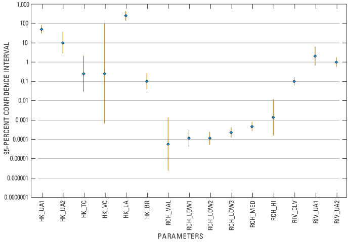
Information regarding parameter uncertainty is provided by the 95-percent linear confidence intervals shown in figure 19 and table 5. Confidence intervals represent the uncertainty in the simulated values that is a propagation of the uncertainty in the estimated parameter values (Poeter and Hill, 1998). A relatively small range indicates there was sufficient information to accurately estimate the parameter value. The logarithmic scale of figure 19 makes it difficult to see the actual size of the confidence interval. To correct this difficulty, figure 20 shows the upper and lower confidence intervals computed as a percentage of the final value. Linear confidence intervals were assumed to adequately approximate the actual nonlinear confidence intervals (Cooley, 1997; Hill, 1998).
The upper and lower 95-percent confidence intervals should be reasonable values. The confidence intervals for hydraulic conductivity (except unit VC) and river conductance parameters spanned a reasonable range, indicating sufficient information exists to estimate the parameter value.
If two parameters are highly correlated, they cannot be uniquely estimated. Parameter correlations range from -1.0 to +1.0, and for any set of parameters, an absolute value greater than 0.95 indicate a potential problem. All correlation coefficients were within acceptable range except the hydraulic conductivity and vertical anisotropy for unit VC.

Comparison of Simulated and Measured Hydraulic Heads
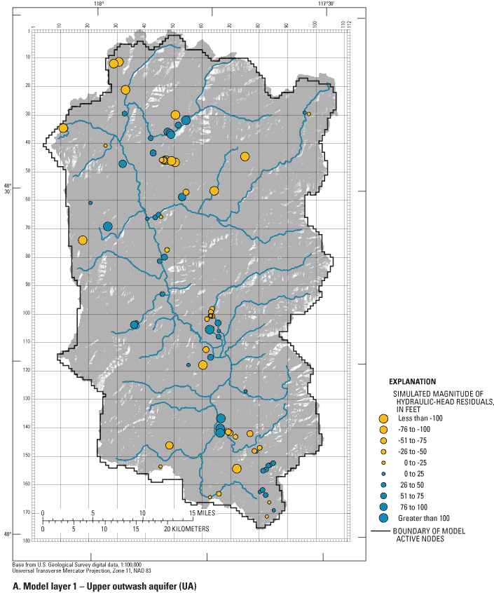
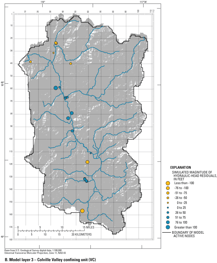
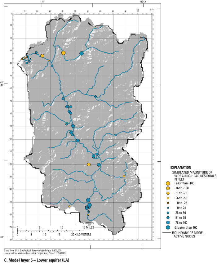
A more traditional and intuitive assessment of model calibration can be achieved by visually comparing the magnitude and spatial distribution of unweighted residuals. Figures 21A-C show the simulated hydraulic-head residuals for units UA, VC, and LA. For simulated hydraulic heads to be acceptable, the distribution of heads and the patterns of flow in units UA, VC, and LA had to match the general water-level distributions and flow patterns measured in the field. Also, root-mean-square (RMS) error of the difference between simulated and measured hydraulic heads in the 161 observation wells, divided by the total difference in water levels in the ground-water system (Anderson and Woessner, 1992, p. 241), had to be less than 10 percent to be acceptable.
The calibrated model produces an RMS error divided by the total difference in water levels (RMSTD) of 4 percent. RMSTD for units UA, VC, and LA, are 3, 3, and 2 percent, respectively. Sixty-one percent of the 161 simulated hydraulic heads exceeded measured heads and the spatial distribution of the hydraulic head residuals show definite patterns of bias. In unit UA, 54 percent of simulated heads exceeded measured heads and these exceedances occurred throughout the model. A more prevalent bias is associated with units VC and LA. Most simulated hydraulic heads along the main Colville River valley floor exceeded the measured hydraulic heads with the exception of heads in unit LA near Kettle Falls. The nonrandom distribution of residuals in hydraulic heads for units VC and LA is a weakness in the final model.
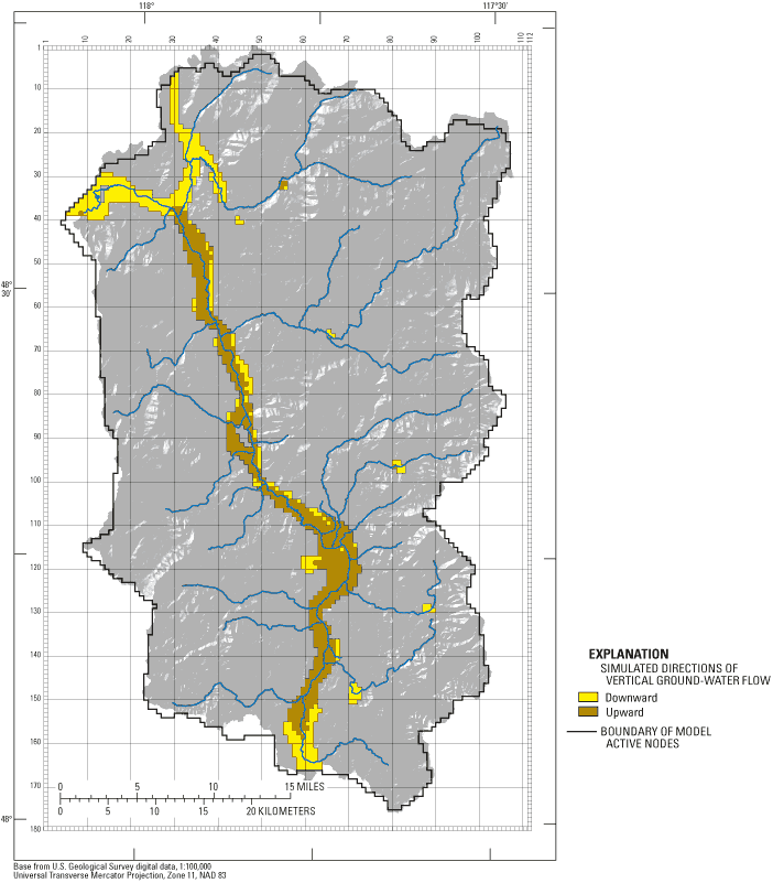
Although a bias exists toward simulated hydraulic heads exceeding measured hydraulic heads, general ground-water-flow patterns indicated by the simulation results match those measured in the field. Kahle and others (2003) measured water levels that indicated downward ground-water flow on the valley floor from near Springdale to near the mouth of Sheep Creek, then upward along much of the valley floor until near Colville, where vertical gradients reverse to downward near the mouth of the watershed at Lake Roosevelt. These general flow patterns are produced by the calibrated model (fig. 22).
Comparison of Simulated and Measured Discharges
The steady-state model calibration benefited greatly from a complete set of seepage measurements (discharge) conducted in September 2001 (fig. 12). These measurements quantified the ground-water discharge to (gaining reach), or recharge from (losing reach) streams. The model was calibrated to 44 discharge measurements. Simulated and measured discharges are shown in table 6 and figure 23. Simulated gains and losses reasonably match the measured discharges but spatial bias does exist. Six of the seven simulated discharge values for the Colville River exceeded measured discharge, including a large discrepancy for the Colville River at Schmidlekofer Road. The measured value for this river reach was a net loss of 5.6 ft3/s (Kahle and others, 2003). The model was unable to reasonably simulate any loss for this reach, instead simulating a net gain of 3.4 ft3/s. Kahle and others (2003) noted that low-flow conditions in the Colville River in 1960 and 1961 were significantly different for this reach than for other reaches along the river. The discharge of the Colville River at Schmidlekofer Road increased by amounts ranging from about 8 to 13 ft3/s during 1960 and 1961. The large difference in discharge was not measured in other reaches along the Colville River. The 1960 and 1961 discharge measurements also indicate that flow conditions can change quickly along the Colville River. Because of this knowledge, the large difference for this reach was considered acceptable. Most tributaries lost flow as the creeks entered the Colville River valley. The model generally simulated slight gains but the absolute values of the residuals were small.
[Postitive values indicate gains. Negative values indicate losses. Abbreviations: ft3/s, cubic foot per second]
| Map No. (figure 12) | Stream | Discharge | ||
|---|---|---|---|---|
| Simulated (ft3/s) |
Measured (ft3/s) |
Residual (ft3/s) |
||
| 1 | Sheep Creek at Forest Center Road, near Springdale | 8.7 | 8.0 | 0.7 |
| 2 | Sheep Creek at mouth, near Springdale | 0.1 | -1.1 | 1.2 |
| 3 | Deer Creek near Springdale | 1.9 | 4.7 | -2.8 |
| 4 | Deer Creek at mouth, near Springdale | 0.1 | -0.5 | 0.6 |
| 5 | Colville River at Betteridge Road, near Valley | 0.9 | 1.9 | -1.0 |
| 6 | Jump Off Joe Creek near Valley | -0.4 | 2.8 | -3.2 |
| 7 | Jump Off Joe Creek at mouth, near Valley | 0.0 | -0.0 | 0.0 |
| 8 | Bulldog Creek near Valley | 2.2 | 2.8 | -0.6 |
| 9 | Bulldog Creek at mouth, near Valley | 5.2 | 4.5 | 0.7 |
| 10 | Waitts Creek near Valley | 0.2 | 0.1 | 0.1 |
| 11 | Waitts Creek at mouth, near Valley | 0.1 | 0.1 | 0.0 |
| 12 | Huckleberry Creek near Valley | 0.5 | 0.5 | 0.0 |
| 13 | Huckleberry Creek at mouth, near Valley | 0.0 | -0.4 | 0.4 |
| 14 | Cottonwood Creek near Chewelah | 0.8 | 2.4 | -1.6 |
| 15 | Cottonwood Creek at mouth, near Chewelah | 2.2 | 0.3 | 1.9 |
| 16 | Sherwood Creek near Chewelah | 0.2 | 0.5 | -0.3 |
| 17 | Sherwood Creek at mouth, near Chewelah | 0.1 | -0.1 | 0.2 |
| 18 | Thomason Creek near Chewelah | -0.3 | 0.9 | -1.2 |
| 19 | Thomason Creek at mouth, near Chewelah | 0.4 | -0.1 | 0.5 |
| 20 | North Fork Chewelah Creek, near Chewelah | 2.7 | 3.7 | -1.0 |
| 21 | South Fork Chewelah Creek, near Chewelah | 0.9 | 3.7 | -2.8 |
| 22 | Chewelah Creek at mouth, near Chewelah | 2.0 | -0.2 | 2.2 |
| 23 | Paye Creek near Chewelah | 0.3 | 3.4 | -3.1 |
| 24 | Paye Creek at mouth, at Chewelah | 1.9 | -0.4 | 2.3 |
| 25 | Colville River at Schmidlekofer, at Chewelah | 3.4 | -5.7 | 9.1 |
| 26 | Blue Creek near Blue Creek | 0.0 | 0.1 | -0.1 |
| 27 | Blue Creek at mouth, at Blue Creek | 0.3 | -0.1 | 0.4 |
| E | Colville River at Blue Creek (station 12408000) | 1.0 | -0.3 | 1.3 |
| 28 | Stensgar Creek near Addy | 1.0 | 0.3 | 0.7 |
| 29 | Stensgar Creek at mouth, at Addy | 0.5 | -0.3 | 0.8 |
| 31 | Addy Creek at mouth, at Addy | 0.0 | -0.1 | 0.1 |
| 32 | Stranger Creek near Addy | 1.3 | 0.2 | 1.1 |
| 33 | Stranger Creek at mouth, near Addy | 0.0 | -0.2 | 0.2 |
| 34 | Colville River at 12 Mile Road, near Addy | 1.4 | -0.5 | 1.9 |
| 35 | Little Pend Oreille River at Arden | 13.3 | 13.6 | -0.3 |
| 36 | Little Pend Oreille River at mouth, at Arden | 0.3 | -4.0 | 4.3 |
| 37 | Colville River at Arden | 0.8 | -0.1 | 0.9 |
| 38 | Haller Creek below Cole Creek, near Arden | 0.5 | 1.0 | -0.5 |
| 39 | Haller Creek at mouth, near Arden | 0.5 | -1.0 | 1.5 |
| 40 | Mill Creek at Douglas Falls, near Colville | 5.3 | 3.8 | 1.5 |
| 42 | Clugston Creek near mouth, near Colville | -0.3 | 0.4 | -0.7 |
| 43 | Mill Creek at mouth, near Colville | -0.1 | -2.3 | 2.2 |
| 46 | Colville River at Greenwood Loop Road, near Kettle Falls | 0.8 | -0.3 | 1.1 |
| J | Colville River at Kettle Falls (station 12409000) | -0.7 | -0.7 | 0.0 |

Figure 23. Simulated and measured discharge of the Colville River, Stevens County, Washington.
Discharge measurements of the tributary upper reaches of the Colville River Watershed created some statistical difficulties with the nonlinear calibration. The accuracy of the measurements was considered excellent and therefore a high weight was assigned to them. The actual discharge values, however, were very small. Fourteen of the 19 measured discharges were less than 2 ft3/s. Large weighted residuals for the discharges in some minor tributaries were considered acceptable.
The upstream tributary discharge measurements were made where the stream enters the Colville River valley floor, and the discharge measured at these locations is presumed to include the total ground-water discharge to the stream for the entire subbasin. No information exists to quantify where the recharge occurs along the stream or the volume of ground water that flows beneath the stream. Small residuals for these locations indicate only that the total streamflow is correct. There is no way to know if all the hydrologic processes of the subbasin are being simulated correctly. Simulations of the subbasins therefore have a large degree of uncertainty and users are cautioned against extending predictions past the appropriate level for the regional model.
For more information about USGS activities in Washington, visit the USGS Washington District home page .
![]()
![]()