Version 1.2
U.S. Department of the Interior
U.S. Geological Survey
This research was supported by the U.S. Department of Defense through the Strategic Environmental Research and Development Program (SERDP)
U.S. Department of the Interior
Gale A. Norton, Secretary
U.S. Geological Survey
Charles G. Groat, Director
U.S. Geological Survey, Reston, Virginia: 2005
This publication is only available online at URL: https://pubs.usgs.gov/sir/2005/5045/
For information on other USGS products and ordering information:
World Wide Web: http://www.usgs.gov/pubprod/
Telephone: 1-888-ASK-USGS
For more information on the USGS—the Federal source for science about the Earth, its natural and living resources,
natural hazards, and the environment:
World Wide Web: http://www.usgs.gov/
Telephone: 1-888-ASK-USGS
Any use of trade, product, or firm names in this publication is for descriptive purposes only and does not imply endorsement by the U.S. Government.
Although this report is in the public domain, permission must be secured from the individual copyright owners to reproduce any copyrighted materials contained within this report.
Scalar magnetic data are often acquired to discern characteristics of geologic source materials and buried objects. It is evident that a great deal can be done with scalar data, but there are significant advantages to direct measurement of the magnetic gradient tensor in applications with nearby sources, such as unexploded ordnance (UXO). To explore these advantages, we adapted a prototype tensor magnetic gradiometer system (TMGS) and successfully implemented a data-reduction procedure.
One of several critical reduction issues is the precise determination of a large group of calibration coefficients for the sensors and sensor array. To resolve these coefficients, we devised a spin calibration method, after similar methods of calibrating space-based magnetometers (Snare, 2001). The spin calibration procedure consists of three parts: (1) collecting data by slowly revolving the sensor array in the Earth's magnetic field, (2) deriving a comprehensive set of coefficients from the spin data, and (3) applying the coefficients to the survey data.
To show that the TMGS functions as a tensor gradiometer, we conducted an experimental survey that verified that the reduction procedure was effective (Bracken and Brown, in press). Therefore, because it was an integral part of the reduction, it can be concluded that the spin calibration was correctly formulated with acceptably small errors.
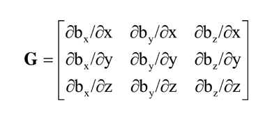
A magnetic gradient is measured by finding the difference between two magnetometer readings and then normalizing the difference with respect to the sensor separation. This forms a gradient in the direction of the line between the two sensors. There are three gradients for a given direction and three linearly independent directions, making nine gradients. These gradients can be arranged into a matrix called a magnetic gradient tensor, mathematically expressed as:
(click on the equation image for a text alternative)
Because both the divergence and curl of a magnetostatic field must equal zero in a sourceless region, this tensor is traceless and symmetric, having only five independent components. The magnetic gradient tensor and three field components comprise a complete description of the magnetic field to the first order. Therefore, a practical tensor magnetic gradiometer will use a spatial array of vector magnetic sensors for differencing and ultimate derivation of the tensor.
For a tensor gradiometer, calibration is particularly important because the ambient field is much larger than the anomalous source fields, and the gradiometer is a differencing device. For example, if two sensors give different readings in a common uniform field, that error will be included in the measured gradient and will be indistinguishable from a true gradient. Furthermore, if the common field is large, the error will be large and will likely overwhelm the gradient being sought. Therefore, the vector sensors must be calibrated to extraordinary levels of precision, which—if obtained by direct-calibration methods—requires costly, specialized facilities and tedious measurements (Graven and Kenny, 1996).
To avoid these difficulties, we derived a method that uses the Earth's field to advantage, similar to the spin methods used on space vehicles (Snare, 2001); hence, the name spin calibration. By slowly turning the sensor array on a carousel in the ambient field, the full range of each sensor axis can be exercised with thousands of data points. This suggests the use of regressions for coefficient derivations. We use two nonlinear regressions: one combines the spin data with scalar base-station magnetometer data to calibrate each of four vector magnetometers individually; the other uses only spin data to rotate the four sensors precisely into a common reference frame.
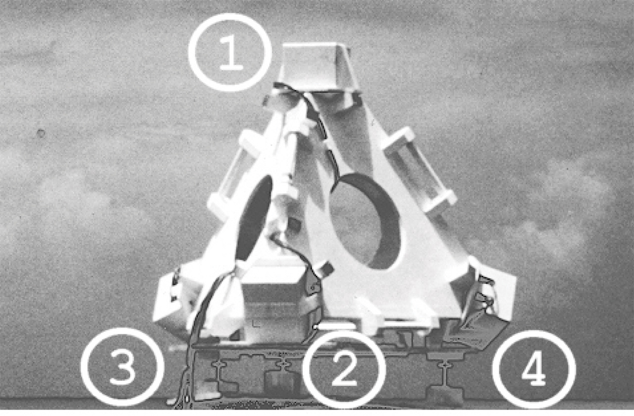
The TMGS consists of two basic units. Figure 1 shows the sensor array called TESSA (tetrahedral em/mag sensor suspension apparatus), which is a 1-m hollow tetrahedron with four triaxial magnetic sensors at its vertices. The sensors are numbered and located inside the protective cases shown in the figure. The magnetometers are ring-core triaxial fluxgates manufactured by Narod Geophysics (Narod, 1987) for use in magnetic observatories by the U.S. Geological Survey (USGS). The second unit (not pictured) is an enclosure that provides a thermally controlled environment for the magnetometer interface electronics. It contains circuitry that measures the temperature of each sensor and samples the magnetometer output. The raw data are sent, via an RS-232 link, to a laptop computer for storage. The TMGS was originally designed for detection of volcano magnetic effects from a stationary observation point (Bracken and others, 1998). Therefore, its size and sensor geometry have not been optimized for UXO applications. However, the spin-calibration procedure developed for this instrument can be applied to any tensor gradiometer system.
|
Figure 1. TMGS sensor array (TESSA) with sensors numbered. |
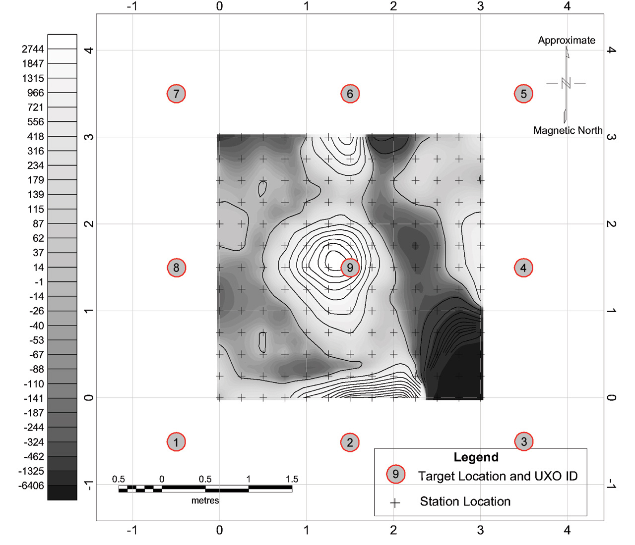
On March 12, 2003, the USGS used the TMGS to perform an experimental survey over a known UXO target at the Standardized UXO Test Site in Yuma Proving Ground, Arizona (YPG). The target was a 60-mm mortar shell buried 0.25 m deep. We collected the data as 10-s stationary observations at five samples per second over a 3-m-square grid centered on the target and having 0.25-m grid cells. Smith and Bracken (2004) describe the survey in detail. Three categories of data were collected on-site: (a) primary measurements including magnetics, position, and attitude; (b) spin calibration measurements; and (c) thermal baseline measurements. Some calibration data used in the reduction procedure were collected in the laboratory.
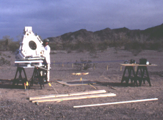
We erected a nonmagnetic turntable calibration apparatus (fig. 2) in an area of known low magnetic gradients near a reference base magnetometer. Plastic trestles were used to elevate the sensor array about 1.5 m above the ground in order to reduce noise from near-surface sources. The turntable was driven by a small, high-torque DC electric motor through a 1:50 reduction gear. The motor and gearbox assembly were about 3 m away from the turntable, where a magnetic interference test confirmed the absence of static and dynamic magnetic noise. The turntable completed one revolution (360 degrees) in 48.5 minutes (8.09 seconds per degree). We chose a low spin rate because the TMGS was not designed for high angular velocities. Four data sets were acquired. In each, TESSA was resting on a different face and completed one revolution.
Figure 2. TESSA on spin-calibration turntable with drive assembly on right connected with nonmagnetic drive belt. |
|
The magnetometers and the sensor array are calibrated using equations that contain the subject coefficients of the spin-calibration regressions. Therefore, we first describe each of three forward calibration equations that are generally applicable to any tensor gradiometer system.
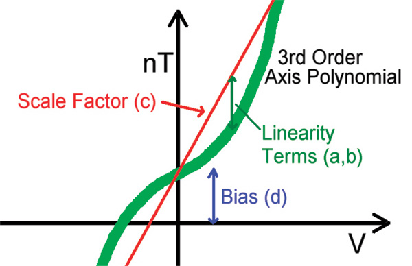
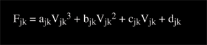
The output voltage of each axis of each magnetometer is converted into magnetic field with a third-order polynomial (axis polynomial). Figure 3 is an exaggerated view showing how the axis polynomial transforms a magnetometer output voltage into a calibrated field component value. The result, Fjk, is the calibrated field component value of the jth axis of the kth sensor; Vjk is the output voltage for the subscripted axis; and ajk, bjk, cjk, and djk are the coefficients to be calculated from the spin data (for calibrating linearity, scale factor, and bias):
(click on the equation image for a text alternative)
|
Figure 3. Coefficients in the axis polynomial. |
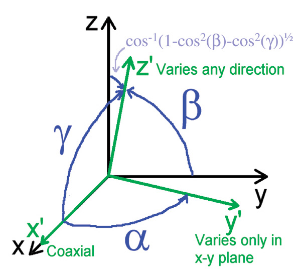
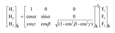
The three calibrated axes of a given magnetometer, which are nominally orthogonal, are aligned into a true orthogonal coordinate system by an orthogonality correction. The result, Hjk, is the aligned jth axis of the kth sensor. The aligning angles, αk, βk, and γk (fig. 4), are to be calculated from the spin data. (Note that the orthogonality matrix in the following equation is inverted.)
(click on the equation image for a text alternative)
Figure 4. Alignment angles used in the orthogonality correction. |
|
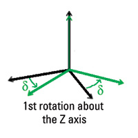
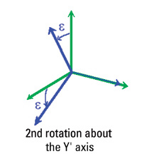
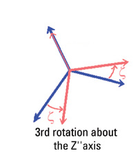
A sensor attitude correction rotates each of the sensors numbered 2, 3, and 4 (fig. 1) into the sensor-1 frame (coordinate system). The sensor-1 frame is nominally the same as the sensor array's frame. The result, Bjk, is the field component value of the jth axis of the kth sensor rotated into the sensor array frame. The attitude correction angles, δk, εk, and ζk (fig. 5), are rotations about the kth sensor's Z, Y′, and Z″ axes, respectively, to be calculated from the spin data:
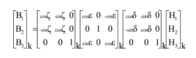
(click on the equation image for a text alternative)
|
Figure 5. Diagram of attitude correction rotations. |
Gradients can then be found by differencing the Bjk. For example, the gradient of the y-component along the line from the 1st sensor to the 4th sensor would be expressed as (B24−B21) ⁄ E, where E is the distance between the sensors. Although gradients calculated in this way can be used to derive the final tensor, it is more easily done analytically by fitting a 3-dimensional function to Bjk.
For a given sensor, the coefficients of its axis polynomial and orthogonality correction are derived simultaneously using a nonlinear regression; each sensor is treated independently. At a given sample point, n, the magnitude of the sensor is derived from the output voltages of its three axes using the axis polynomial and orthogonality equations. The regression finds the coefficients (ajk, bjk, cjk, djk and αk, βk, γk) by fitting these derived signals to measured responses (In), recorded by the base magnetometer, according to this equation:
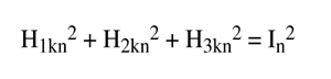
(click on the equation image for a text alternative)
A second regression is then performed to obtain the attitude correction coefficients (δk, εk, ζk). The Hjkn are first calculated using the coefficients found in the first regression. At a given sample point, n, sensor 2, 3, or 4 is rotated into the sensor-1 frame using the attitude correction equation. The resulting unit field vector (Bkn ⁄ Bkn) is then dotted with the unrotated unit field vector of sensor 1 (H1n ⁄ H1n). The regression finds the coefficients by fitting the dot product to 1 (minimizing the angle between unit vectors), mathematically collineating the two coordinate systems, according to this equation:
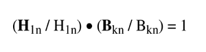
(click on the equation image for a text alternative)
Before starting either regression, all coefficients are given initial values equal to their nominal values. For the axis polynomial, the nominal values are all zero except for the scale factor, cjk which should be set to the nominal scale factor of the magnetometer being used—in our case 100 nT/V. The orthogonality aligning angles are nominally 90°. The attitude-correction angles depend on the geometry of the sensor array. Examination of figure 5 may assist in deriving values for a particular system.
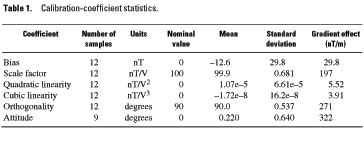
After performing the spin calibration and running the data through the regression, the derived coefficients showed a reasonably small amount of scatter about the nominal values. In table 1, statistics are given for the 12 samples (attitude has only 9 samples) in each category of coefficients. The nominal values are close to the mean values, which is to be expected. The standard deviations also appear reasonable and are consistent with the engineering quality of the system. The gradient effect shows the magnitude of a false gradient that would be superimposed on a typical gradient measurement if the coefficient for one of two differenced sensors had an error equal to the standard deviation and the coefficient for the other sensor had no error. The gradient effect is reported in nT/m with a separation of 1 m, assuming a 50,000-nT ambient field. The impact of the gradient effect is fully realized when the sensor platform undergoes large attitude variation.
The gradient effect shows that there is a wide range in significance of the various coefficients, with the linearity terms being least and the attitude correction greatest. However, all of the coefficients are significant by comparison to the experimental survey's central anomaly shown in figure 6. The data reduction (Bracken and Brown, in press), which included this spin calibration, yielded a 14-nT/m target anomaly (derived from the 3,000 nT3 ⁄ m3 peak in fig. 6). Consequently, if the linearity terms had been neglected, the anomaly could have been severely degraded. Had any other coefficients been neglected in the spin calibration, the anomaly could have been obliterated. Furthermore, even a small error in some of the coefficients could have destroyed the anomaly. For example, a 0.02-degree attitude error would translate into a 20 nT/m false gradient and overwhelm the target anomaly. Therefore, because the anomaly in figure 6 was derived by a reduction that included the spin calibration as an essential sequential processing step, it can be concluded that the spin-calibration procedure works and produces reasonably accurate results.
We expect to perform a rigorous analysis of the spin-calibration results to demonstrate attainable accuracy levels. Anticipated improvements to the TMGS will allow spin calibration data to be acquired more rapidly; this will also be investigated. Finally, it is well known that fluxgate magnetometers have significant thermal dependencies. We therefore expect many of the spin-calibration-derivable coefficients to be functions of temperature. These functions may be estimated by performing spin calibrations at a variety of temperatures.
This research was supported wholly by the U.S. Department of Defense through the Strategic Environmental Research and Development Program (SERDP). We acknowledge YPG personnel for facilitating our work at the Standardized UXO Test Site and Professor Yaoguo Li of Colorado School of Mines for providing consultation.
Manuscript approved for publication February 24, 2005
Published in the Central Region, Denver, Colorado
Editing, layout, photocomposition—Richard W. Scott, Jr.
Graphics by the authors
Document Accessibility: Adobe Systems Incorporated has information about PDFs and the visually impaired. This information provides tools to help make PDF files accessible. These tools convert Adobe PDF documents into HTML or ASCII text, which then can be read by a number of common screen-reading programs that synthesize text as audible speech. In addition, an accessible version of Acrobat Reader 6.0, which contains support for screen readers, is available. These tools and the accessible reader may be obtained free from Adobe at Adobe Access.
| AccessibilityFOIAPrivacyPolicies and Notices | |
| |
|