
Prepared in cooperation with the U.S. Environmental Protection Agency
Two-Dimensional Resistivity Methods
Two-Dimensional Resistivity Investigation
Figure 1. Location of North Cavalcade Street site.
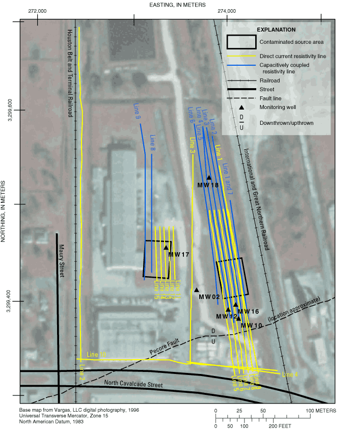
Figure 2. Map of the North Cavalcade Street site showing the direct current...
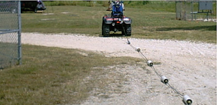
Figure 3. Photograph showing the Geometrics OhmMapper capacitively coupled ...
Figure 4. Photographs showing (A) a stainless steel electrode connected to ...
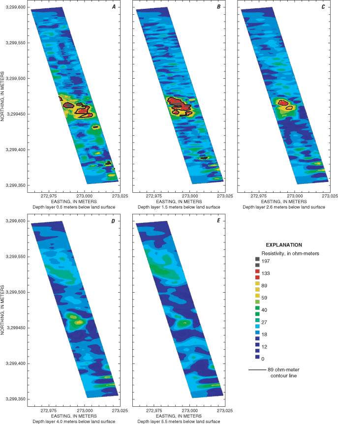
Figure 5. Two-dimensional plan view of depth layers showing the inversion r...
Figure 6. Sections showing inversion results of capacitively coupled resist...
Figure 7. Sections showing inversion results of capacitively coupled resist...
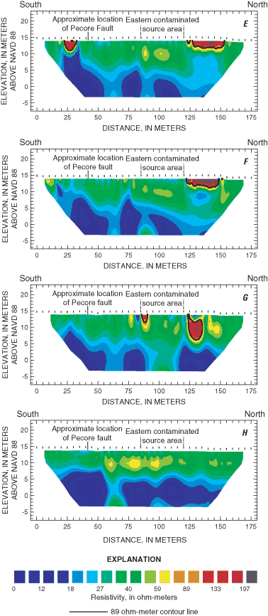
Figure 8. Sections showing inversion results of direct-current resistivity ...
Figure 8. Sections showing inversion results of direct-current resistivity ...
Figure 8. Sections showing inversion results of direct-current resistivity ...
Figure 9. Sections showing (A) forward model, (B) inversion result of forwa...
Figure 9. Section showing (D) forward model, (E) inversion result of forwar...
Figure 9. Section showing (G) forward model, (H) inversion result of forwar...
Figure 9. Section showing (J) forward model, (K) inversion result of forwar...
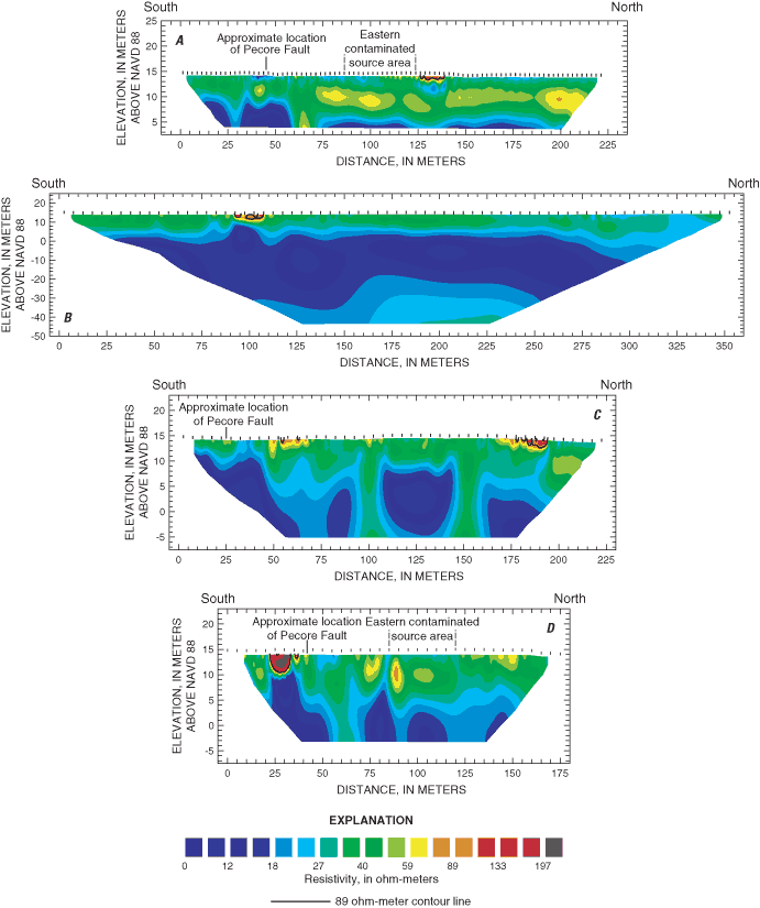
Figure 10. Sections showing interpretation of direct-current resistivity in...
Figure 10. Sections showing interpretation of direct-current resistivity in...
Figure 11. Map of North Cavalcade Street site showing areas of resistive an...
Appendix 1. Summary of features in interpretation sections in the North Cav...
| Multiply | By | To obtain |
|---|---|---|
| Length | ||
| inch (in.) | 2.54 | centimeter (cm) |
| foot (ft) | 0.3048 | meter (m) |
Vertical coordinate information is referenced to the North American Vertical Datum of 1988 (NAVD 88).
Horizontal coordinate information is referenced to the North American Datum of 1983 (NAD 83).
Elevation, as used in this report, refers to distance above the vertical datum.
The North Cavalcade Street site was first developed for wood treating in 1946. By 1955, pentachlorophenol wood preservation services and other support facilities, such as creosote ponds, pentachlorophenol and creosote storage structures, various tanks, lumber sheds, a treatment facility, and other buildings had been added. In 1961, the property was closed. To protect public health and welfare and the environment from release or threatened releases of hazardous substances, the U.S. Environmental Protection Agency added the North Cavalcade Street site to the National Priorities List on October 5, 1984. Between September 1985 and November 1987, the U.S. Environmental Protection Agency conducted a remedial investigation which, through exploratory drilling, determined the locations of two contaminated source areas and a normal fault. During August 2003, the U.S. Geological Survey, in cooperation with the U.S. Environmental Protection Agency, conducted a two-dimensional (2D) resistivity investigation at the North Cavalcade Street site to provide additional characterization of the dense non-aqueous phase liquids and the lithologies that can influence contaminant migration. The 2D resistivity investigation used a capacitively coupled (CC) resistivity method as a reconnaissance tool to locate geophysical anomalies that could be associated with possible areas of creosote contamination. The inversion results of the CC resistivity survey identified resistive anomalies in the subsurface near the eastern and western contaminated source areas. A direct-current (DC) resistivity survey conducted near the CC resistivity survey confirmed the occurrence of subsurface resistive anomalies. The inversion results of the DC resistivity survey were used to define the subsurface distribution of resistivity at each line.
Forward modeling was used as an interpretative tool to relate the subsurface distribution of resistivity from four DC resistivity lines to known, assumed, and hypothetical information on subsurface lithologies. The final forward models were used as an estimate of the true resistivity structure for the field data. The forward models and the inversion results of the forward models show the depth, thickness, and extent of strata as well as the resistive anomalies occurring along the four lines and the displacement of strata resulting from the Pecore Fault along two of the four DC resistivity lines. Ten additional DC resistivity lines show similarly distributed shallow subsurface lithologies of silty sand and clay strata. Eight priority areas of resistive anomalies were identified for evaluation in future studies. The interpreted DC resistivity data allowed subsurface stratigraphy to be extrapolated between existing boreholes resulting in an improved understanding of lithologies that can influence contaminant migration.
The study area referred to as the North Cavalcade Street site is about 1 mile southwest of the intersection of Loop 610 North and U.S. 59, Houston, Harris County, Texas (fig. 1). The North Cavalcade Street site was first developed for wood treating by the Houston Creosoting Co., Inc. (HCCI) in 1946. HCCI increased its capabilities in 1955 by adding pentachlorophenol (PCP) wood preservation services and other support facilities, such as creosote ponds, PCP/creosote storage structures, various tanks, lumber sheds, a treatment facility, and other buildings. The property was closed in 1961 and sold in 1964 to Monroe Ferrell Concrete Pipe Company. Since that time, no industrial activity has taken place on the North Cavalcade Street site (CH2M Hill, 2003). To protect public health and welfare and the environment from release or threatened releases of hazardous substances, the U.S. Environmental Protection Agency (USEPA) proposed that the North Cavalcade Street site be added to the National Priorities List on October 5, 1984. By June 10, 1986, the site was added to the final list (CH2M Hill, 2003). More detailed information on the location and history of the North Cavalcade Street site is provided by the USEPA (2003).
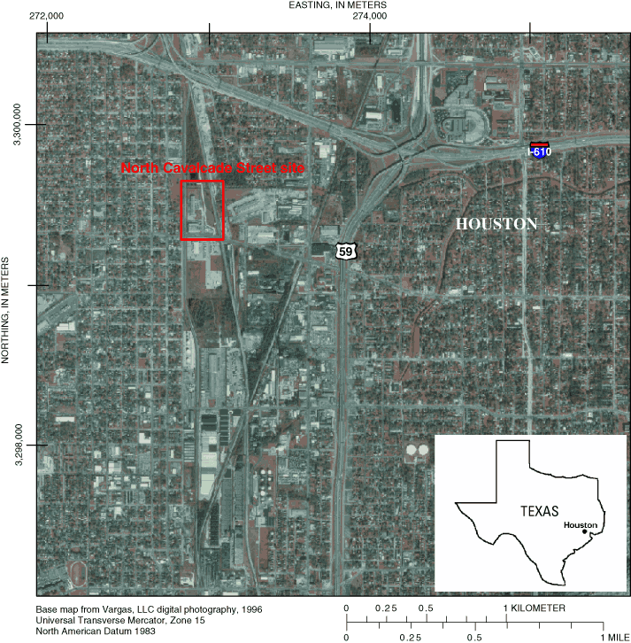
Figure 1. Location of North Cavalcade Street site.
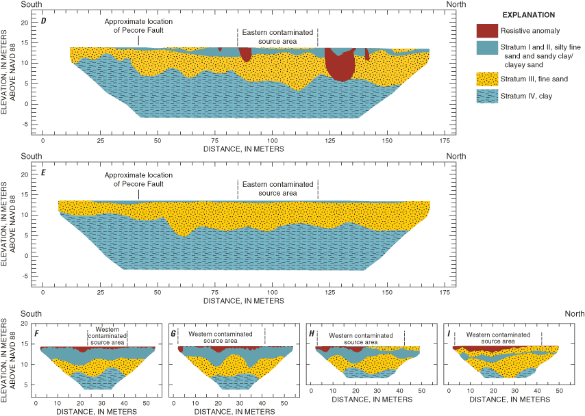
The USEPA initially responded by conducting a Remedial Investigation (RI) between September 1985 and November 1987 to characterize the North Cavalcade Street site. Air, sediment, soil, surface-water, and ground-water samples were collected during the RI and analyzed for toxic substances associated with wood preservation sites (U.S. Environmental Protection Agency, 2003). During the RI, 15 borings, ranging in depth from 15 to 80 feet, were collected and used to describe the basic stratigraphy of the North Cavalcade Street site. The locations of two contaminated source areas and a normal fault (Pecore Fault) that trends generally east to west near the southern boundary were identified during the RI (figure 2-4 and exhibit 2, Camp Dresser & McGee Inc. (CMD), 1987). These features were digitized and are included in figure 2 of this report.
According to CH2M Hill (2003, p. 8), "The USEPA released a Record of Decision (ROD) in 1988 which required onsite biological treatment of soils containing carcinogenic polyaromatic hydrocarbons (PAHs). The ROD also required for groundwater to be extracted and treated until all non-aqueous phase liquids (NAPLs) were completely removed. However, since the first five year review of the ROD (July 1998), additional site characterization has confirmed that the dense non-aqueous phase liquid (DNAPL) extends to a deeper interbedded sand aquifer at 25 to 40 feet below surface." Typically, additional environmental site characterization used to determine depth and extent of DNAPLs and the lithologies in which they are contained has been through exploratory drilling. The accuracy of environmental site characterization is dependent on the number of sample points or borings and the ability to interpolate between these sample points (American Society for Testing and Materials, 1999). Interpolation between sample points may be poorly constrained and lead to an inaccurate site characterization. An alternative approach is to combine surface geophysical methods with a drilling program. Surface geophysical measurements can be made relatively quickly, are minimally intrusive, and enable interpolation between known points of control (American Society for Testing and Materials, 1999). To provide additional characterization of the DNAPL and the lithologies that can influence contaminant migration, the U.S. Geological Survey (USGS), in cooperation with the USEPA, conducted a two-dimensional (2D) resistivity investigation, using capacitively coupled (CC) and direct-current (DC) resistivity methods, at the North Cavalcade Street site during August 2003.
This report describes the methods and results of a 2D resistivity investigation of the North Cavalcade Street site conducted in August 2003. The purpose of this report is to document the inversion results of the CC and DC resistivity surveys, forward modeling and interpretation of four selected lines of DC resistivity data using lithologic descriptions of existing boreholes, and the interpretation of 13 DC resistivity lines at the North Cavalcade Street site.
The geology of the North Cavalcade Street site consists of interbedded clays, silts, and sands associated with the Beaumont Formation, with a ground-water level approximately 4 feet below land surface (U.S. Environmental Protection Agency, 2003). The Five Year Review Report by CH2M Hill (2003) indicated two water-bearing units underlying the North Cavalcade Street site: the shallow sand aquifer and the interbedded sand aquifer. The shallow sand aquifer was described as occurring at a depth of about 15 feet below land surface and is hydraulically connected to the interbedded sand aquifer, consisting of interbedded silty sand and clay, ranging in depth from about 25 to 40 feet below land surface (CH2M Hill, 2003). These water-bearing units are underlain by a regional confining clay that is about 100 feet thick and serves as a barrier to the downward migration of contaminants (CH2M Hill, 2003).
The basic stratigraphy of the North Cavalcade Street site was characterized in the RI as containing four distinct soil strata. Although there is local variability in the depth and thickness of individual strata, the general depth and description of each stratum are as follows: stratum I, land surface to about 2 feet below land surface, fill consisting of silty fine sand; stratum II, approximately 2 to 10 feet below land surface, soft to very stiff sandy clay and clayey sand; stratum III, about 10 to 20 feet below land surface, medium dense to dense fine sand; and stratum IV, approximately 20 to 80 feet below land surface, very stiff to hard clay and silty clay with sand and silt layers (Camp Dresser and McGee Inc., 1987).
Active land subsidence has been accelerated during recent years because of extensive withdrawal of ground water and petroleum supplies in the Greater Houston Area (Camp Dresser and McGee Inc., 1987). The only known land subsidence feature that has occurred at the North Cavalcade Street site is the Pecore Fault. It is a normal "down-to-the-north" fault, meaning that units on the north side of the fault plane are slipping down relative to the units on the south side. The Pecore Fault is considered a lateral barrier that could prevent the southward migration of contaminants in some of the shallow aquifer units (U.S. Environmental Protection Agency, 2003).
Surface geophysical methods provide a relatively quick and inexpensive means to characterize the subsurface (Powers and others, 1999). Surface geophysical methods measure the physical properties of the subsurface such as electrical conductivity or resistivity, dielectric permittivity, magnetic permeability, density, or acoustic velocity. These methods can be influenced by chemical and physical properties of soil, rock, and pore fluids. Interpretations from these measurements can be used to image the distribution of physical properties in the subsurface (American Society for Testing and Materials, 1999).
Electrical surface geophysical methods can be used to detect changes in the electrical properties of the subsurface. The electrical properties of soils and rocks are determined by water content, mineralogical clay content, salt content, porosity, and the presence of metallic minerals. However, typically the resistivity of the water has a larger effect on the bulk resistivity than the soil or rock type. Variations in these electrical properties of soils and rocks, either vertically or horizontally, produce variations in the electrical signature measured by surface geophysical tools. Changes in the received signal can be related to changes in the composition, extent, and physical properties of the soils and rocks within the subsurface, to the extent that differences in lithology or rock type are accompanied by differences in resistivity (U.S. Army Corps of Engineers, 1995). However, to effectively detect these differences there must be a contrast in the property measured. The target to be detected or geologic feature to be defined must have properties significantly different from "background" conditions (American Society for Testing and Materials, 1999).
Contaminants can change the electrical properties of the subsurface, resulting in a measurable contrast with background conditions. Guy and others (2000) demonstrated the potential for using surface geophysical methods to identify the extent and variation with depth of electrically resistive anomalies at a creosote pressure-treating site in Ohio. The study located resistive anomalies in the subsurface, which were confirmed to be creosote contamination through exploratory sampling.
For this study, a 2D-resistivity investigation of the North Cavalcade Street site was conducted using CC and DC resistivity surveying and inverse modeling methods to determine the possible extent and depth of creosote contamination in the subsurface. The DC resistivity survey also was used to extrapolate stratigraphy between existing boreholes using inverse and forward modeling methods. These combined methods were used to develop an improved understanding of lithologies that can influence contaminant migration. Lithologic descriptions from geologist logs for six monitoring wells (fig. 2) were supplied by the USEPA to aid in the interpretation of resistivity data.
CC resistivity measures apparent resistivity of the earth through four antennas in a dipole-dipole array (Loke, 2002a). In this dipole-dipole array, two antennas are connected to a transmitter and are used as a transmitting dipole. The remaining two are connected to a receiver and are used as the receiving dipole (Baker, 2003). By alternating voltage in the transmitting dipole, an alternating-current (AC) is coupled to the earth at a particular frequency. The electrical current coupled to the earth causes voltages to be produced, which are measured by the receiving dipole. Variations in the resistivity of the subsurface alter the voltage that is returned. Resistance is calculated by dividing the voltage measured by the receiver dipole by the current from the transmitting dipole. The apparent resistivity of the subsurface was calculated by multiplying the resistance value by a geometric correction that is determined by the geometry and the spacing of the array (Loke, 2002a). A greater depth of investigation is achieved by increasing the distance between the midpoints of the transmitter and receiver (Baker, 2003). This is achieved by lengthening the dipole cables (antennas) or the distance between the transmitter and receivers.
The Geometrics TR4 OhmMapper (fig. 3), a mobile resistivity measuring system, was used to perform the CC resistivity survey. This system uses one transmitter dipole and four receiver dipoles, which establish electrical contact with the earth through capacitive coupling. The transmitter dipole and receiver dipoles were towed across the ground surface behind an all-terrain vehicle (ATV) as resistivity data were continuously collected in a series of nine lines (fig. 2). A sub-meter accuracy, differentially corrected global positioning system (DGPS), interfaced directly with the logging unit of the OhmMapper, was used to collect continuous locational data. The use of the ATV and the DGPS provide the user with the ability to characterize the subsurface over a large area in a relatively short amount of time (Geometrics, 2004).
Using the Wenner-Schlumberger array (Loke, 2002b), DC resistivity measurements were made by inducing direct current into the ground through two current electrodes and measuring the resulting voltage between two potential electrodes located between the current electrodes. Resistance was then calculated by dividing the measured voltage by the induced current. The apparent resistivity of the subsurface was calculated by multiplying the resistance value by a geometric correction that is determined by the geometry and the spacing of the electrode array.
The electrodes were connected to electrode terminals built into multi-conductor cables (fig. 4a) and joined by an automatic switching unit (fig. 4b). These units are designed to automatically perform pre-defined sets of resistivity measurements using multiple electrodes to facilitate more rapid data collection (Stanton and others, 2003).
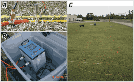
The DC resistivity data at the North Cavalcade Street site were collected along 15 lines (fig. 2) using an IRIS Syscal R1 Plus switching unit (fig. 4b). Using four electrodes at a time, the unit switches among a combination of four sets of multi-conductor cables (fig. 4c) to collect multiple points from a single layout. Electrodes were typically placed every 5 meters, and spacing was decreased where needed to accommodate field conditions or to increase data density. After the initial section of data was collected, the first cable of 18 electrodes was moved ahead of the survey line. A partial section of data was then collected using the previous 56 electrodes (electrodes 19-72) and the 18 electrodes (electrodes 73-90) that were just moved. This process, known as the roll-along technique, was continued until all data along the desired line length were collected. The data from the roll-alongs were combined into a single dataset during processing.
Field measurements of apparent resistivity were collected using both CC and DC resistivity methods. The field measurements of apparent resistivity were calculated by multiplying the resistance value by a geometric correction. The geometric correction is based on the arrangement of the current electrode or transmitter and the potential electrode or receiver in relation to each other (Degnan, 2001). Apparent resistivity is not the true resistivity because a resistively homogeneous, isotropic subsurface is assumed (Powers, 1999). To estimate the true resistivity or the resistivity structure where the subsurface is heterogeneous and/or anisotropic, the apparent resistivity data were processed using an inverse modeling software program (Loke, 2002a). Apparent resistivity data were processed using either the 2D (RES2DINV software version 3.54; Loke 2004a) or three-dimensional (3D) version (RES3DINV software version 2.14; Loke, 2004b) of the software. The results from this program were used to generate 2D sections of resistivity data referred to as inverted field datasets or inversion results. The inversion results were used to characterize the subsurface resistivity distribution.
Forward modeling was used to predict the system response based on known, assumed, or hypothetical knowledge of the system parameters. In the case of resistivity forward modeling, the system response is the apparent resistivity and the system parameters are the true resistivity structure (F.D. Day-Lewis, U.S. Geological Survey, written commun., 2004). Forward models use a specified 2D grid of rectangular model blocks. These model blocks were assigned resistivity values that represent the true resistivity structure. The true resistivity structure used in each forward model was estimated by comparing the lithologies identified in the available nearby borehole information to inversion results and creating forward modeling units (FMU). An FMU is a group of model blocks representing a particular lithology and stratum or feature of interest (anomaly). The resistivity of an FMU can contain multiple resistivity values to account for variations of lithology in the stratum or an anomaly. The rectangular grid of model blocks or estimate of true resistivity structure was used to calculate synthetic apparent resistivity values.
Forward models were created for lines 1, 2, 6, and 11 using RES2DMOD software version 3.01 (Loke, 2002b). The input model grids were initially constructed in RES2DMOD using lithologically distinct strata identified in available boreholes to define the extent, depth, and thickness of each FMU. Resistivity values were estimated for each FMU using resistivity values from the inversion results of the DC resistivity field data. In some cases data from the available boreholes were not sufficient and the depths and thicknesses of FMUs were estimated. Following construction, synthetic apparent resistivity values were calculated for the forward models using RES2DMOD. These synthetic apparent resistivity values were processed using RES2DINV following the same procedures used in processing the field data. If the inversion results of the synthetic data did not match the field data inversion results, the forward model was modified by adjusting the depths or the resistivity values assigned to the FMUs. The refined forward model was then used to recalculate synthetic apparent resistivity values, which were reprocessed using RES2DINV. A forward model solution was reached when the synthetic data inversion results and inversion results of the field data approximately matched. The final forward model grid was used to provide a detailed, non-unique interpretation of lithologically distinct strata and anomalies occurring along lines 1, 2, 6, and 11 (Degnan and others, 2001). Based on the responses of the forward modeling of lines 1, 2, 6, and 11, lines 3, 5, 7 through 9, and 12 through 15 were interpreted similarly.
Lines 1 and 2 were selected because they were near the eastern and western site boundaries. Forward models of these lines were used to define the relation between the resistivity structure and the approximate lithologic structure along the eastern and western site boundaries. Lines 6 and 11 were selected to aid in the interpretation of lines collected in the eastern and western contaminated source areas. Forward models of these lines were used to define the resistivity structure of anomalies and the lithologic structure in which they were located.
CC resistivity data were collected in the eastern and western contaminated source areas. The data were collected in a series of nine lines. Lines 1 through 7, trending south to north (fig. 2), targeted the eastern contaminated source area. Lines 1 and 7 (represented as a single line on the eastern-most side of the contaminated zone) were overlapping lines to evaluate the repeatability and quality of the CC resistivity surveying method. Data from lines 1 through 7 were combined into one dataset in the software Magmap 2000 (Geometrics, Inc., 2002) and inverted as a 3D dataset. The inversion results from lines 1 through 7 are presented in a series of five horizontal depth layers representing layers 0.5, 1.5, 2.6, 4.0, and 5.5 meters below land surface. Each depth layer (fig. 5) was analyzed to identify resistivity anomalies. Resistivity values greater than 89 ohm-meters were identified as anomalously high resistivity values. A contour line at the value of 89 ohm-meters was used to identify areas containing anomalously high resistivity data. The locations of these resistive anomalies were used to determine the location of the DC resistivity survey.
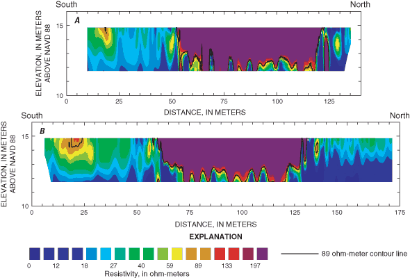
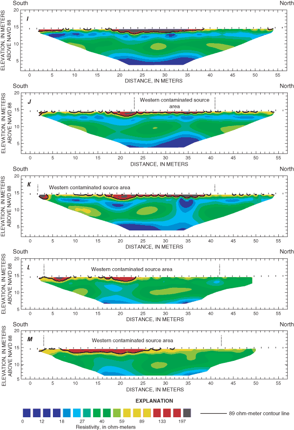
The western contaminated source area was confined by a fence to the south and east, a building to the west, and a parking lot to the north. These features decreased maneuverability of the towed array; therefore, data only were collected along lines 8 and 9 in this area (fig. 2). Because data from only two lines were collected in the western contaminated source area, the data could only be inverted as two 2D datasets. Lines 8 and 9 are presented as vertical 2D sections within the site. Data from lines 8 and 9 (fig. 6) were collected as continuous datasets through the parking lot north of the western contaminated source area. Data collected in the parking lot showed a highly resistive anomaly (fig. 6) that was probably an effect of the concrete in the parking lot.
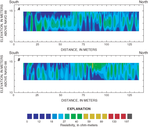
To evaluate the repeatability of the OhmMapper data, data from two overlapping lines were compared. Data along line 1 were collected by profiling from south to north along the eastern edge of the eastern contaminated source area. After data along lines 2 through 6 were collected, data at line 1 were recollected as line 7 by profiling from south to north. Lines 1 and 7 (fig. 7) produced similar datasets with small differences between the two resistivity profiles. Variations in the datasets were probably caused by the difficulty of towing the array in exactly the same path as the original line. The similarities between these two datasets indicate that the results of the CC resistivity were reproducible.
Data from lines 1 through 4 and 10 were collected to define the extent and thickness of strata surrounding the North Cavalcade Street site (fig. 2). Lines 1, 3, and 10 also were positioned to collect data near the Pecore Fault. Resistive anomalies identified in the inversion results of the CC resistivity data (figs. 5-6) were used to aid in the placement of 10 additional DC resistivity lines (fig. 2). Data from lines 5 through 9 were collected near the eastern contaminated source area and data from lines 11 through 15 were collected near the western contaminated source area to further define resistive anomalies identified in the CC resistivity data and to provide additional information on the extent and thickness of the strata associated with these resistive anomalies. Lines 5 through 9 also were positioned to collect data near the approximate location of the Pecore Fault (based on fig. 2-4 of Camp Dresser & McGee Inc. (CMD), 1987).
The inversion results of lines 1 through 3, 5 through 9, and 11 through 15 (fig. 8) were displayed by plotting vertical 2D sections of the resistivity data for each line. A contour line at the value of 89 ohm-meters was used to identify areas containing anomalously high resistivity data. The inversion results from lines 4 and 10 were eliminated due to poor quality data resulting from underground utilities located immediately north of North Cavalcade Street.
The true resistivity structure was estimated for DC resistivity lines 1, 2, 6, and 11 using known, assumed, and hypothetical knowledge to create forward models. By comparing known lithologic information from geologist logs of six monitoring wells (fig. 2) to the inversion results of the DC resistivity data, FMUs representing strata identified in the RI (Camp Dresser & McGee Inc. (CMD), 1987) were developed and used as an initial forward model. Resistivity values were estimated for each FMU using resistivity values from the inversion results of the DC resistivity field data. These values were altered as necessary to improve the visual match between the inverted field resistivity and model sections. The FMUs of strata III and IV were divided into two resistivity values to better simulate the variation of the lithology within each stratum. The final FMUs that were used to represent strata identified in the RI are as follows: silty fine sand and sandy clay/clayey sand deposits (strata I and II) were modeled using a resistivity of 20 ohm-meters, fine sand deposits were modeled with resistivity values of 50 and 75 ohm-meters (stratum III), and clay deposits (stratum IV) were modeled with resistivity values of 5 and 15 ohm-meters (fig. 9). Initial forward models for line 2 modeled stratum IV as a continuous low resistivity (5 and 15 ohm-meters). However, this continuous low resistivity FMU did not adequately simulate the increase in resistivity at approximately -28 meters elevation between 160 and 245 meters along the line 2 (fig. 8b). No borehole data were available to determine the cause for the increase in resistivity at that depth along line 2. Therefore, another FMU of unknown lithology was used in line 2. To estimate the resistivity structure of this feature, several configurations of the depth, thickness, extent, and resistivity were simulated. An FMU with a resistivity of 1,000 ohm-meters was determined to best represent this increase in resistivity.
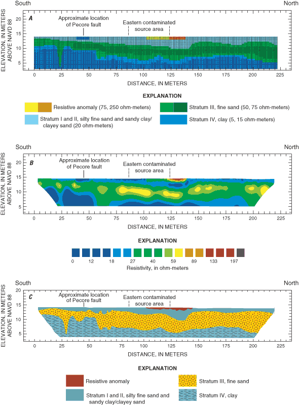
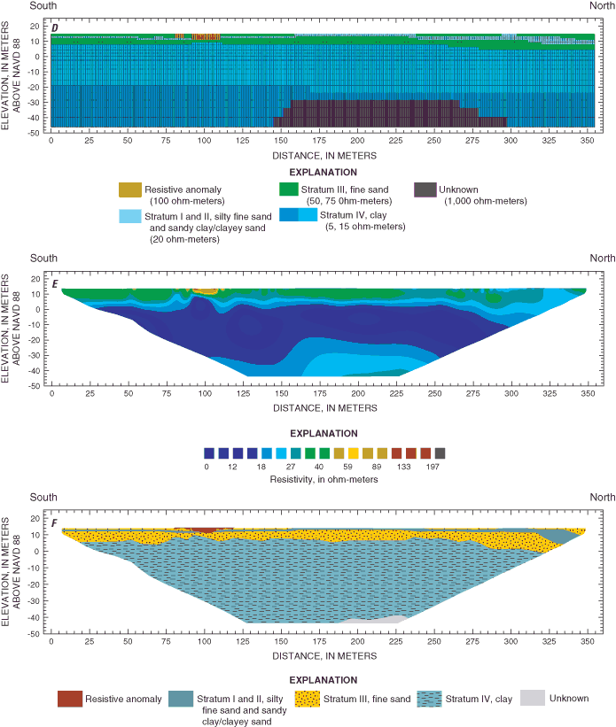
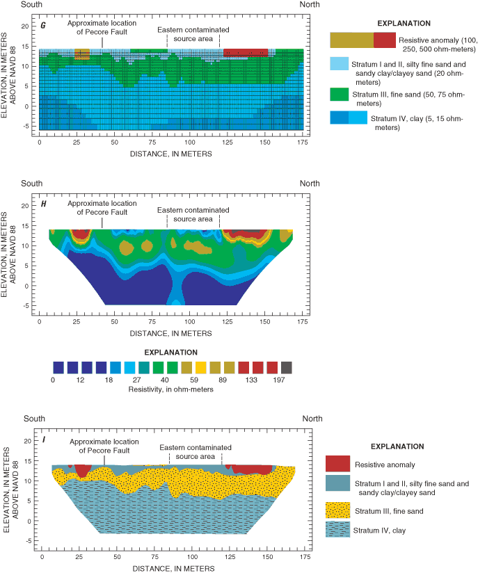
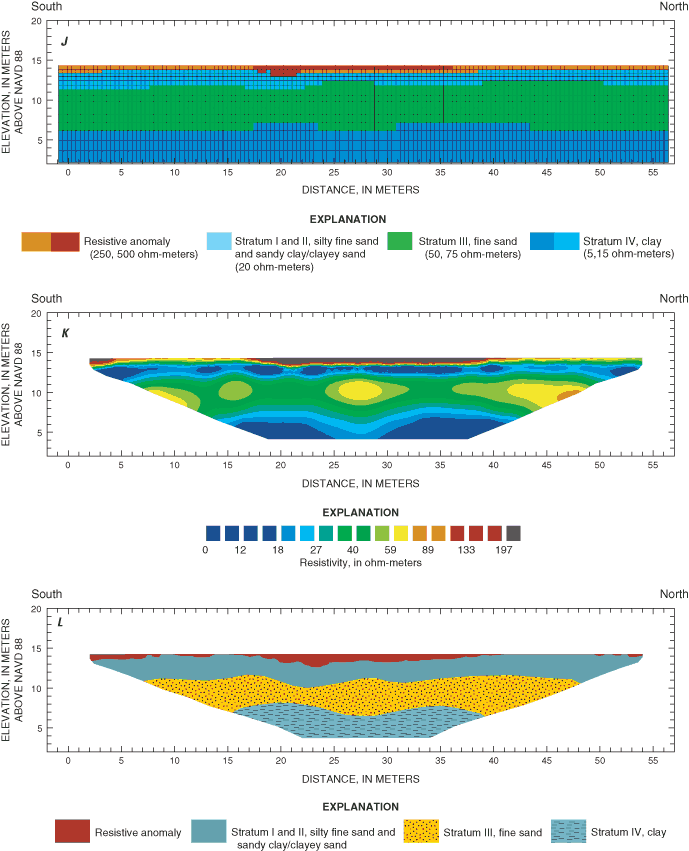
After the forward model representing the different strata was developed for DC resistivity data along lines 1, 2, 6, and 11, the displacement observed for the Pecore Fault was incorporated into the forward models for lines 1 and 6. The RI defined the approximate location of the Pecore Fault along the North Cavalcade Street site. The RI also indicated that lithologic units on the north side of the fault plane are slipping down relative to the lithologic units on the south side. To adequately forward model DC resistivity lines 1 and 6 assumptions about the exact location of the Pecore Fault and the amount of displacement along lines DC resistivity lines 1 and 6 were made to estimate the true resistivity structure. These assumptions were tested primarily using the forward model for DC resistivity line 1. When the inversion results of both the forward model data and the field data for line 1 approximately matched, a forward model for line 6 was developed and tested using the forward model for line 1 as a starting point.
Resistive anomalies also were forward modeled in lines 1, 2, 6, and 11. Because "ground truthing" of the inversion results of the CC and DC resistivity data was not part of this study, resistive anomalies identified in the inversion results of the DC resistivity data for lines 1, 2, 6, and 11 (figs. 8A, 8B, 8E, and 8I) were forward modeled by hypothesizing the true resistivity structure. To determine the configuration of depth, thickness, extent, and resistivity of resistive anomalies used in the forward models of DC resistivity lines 1, 2, 6, and 11, several hypotheses were tested independently for each line using an iterative forward modeling process. FMUs representing resistive anomalies were modeled with resistivity values of 75, 100, 250, and 500 ohm-meters. When resistive anomalies in the inversion results (fig. 9B, 9E, 9H, and 9K) of a forward model closely matched resistive anomalies of the inversion results of the field data, the resulting forward model (fig. 9A, 9D, 9G, and 9J) was used to develop the interpretation of each line (fig. 9C, 9F, 9I, and 9L).
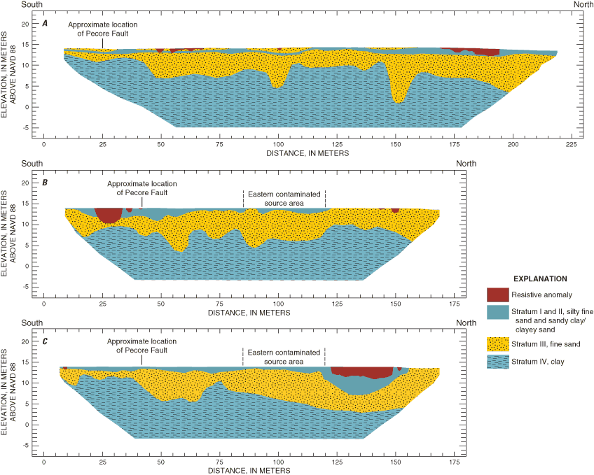
The final forward models for lines 1, 2, 6, and 11 were used as an estimate of the true resistivity structure occurring along those lines. Using these forward models as the estimated true resistivity structure, features showing similar characteristics in lines 3, 5, 7 through 9, and 12 through 15 were interpreted similarly. The forward model, inversion result of the forward model, and interpretation for line 1 were used to interpret strata and resistive anomalies occurring in the subsurface distribution of resistivity of line 3 (fig. 10A). The forward model, inversion of the forward model, and interpretation for lines 6 and 11 were used to interpret strata and resistive anomalies in the subsurface distribution of resistivity for DC resistivity lines 5, 7, 8, and 9, near the eastern contaminated source area (fig. 10B, 10C, 10D, and 10E) and DC resistivity lines 12, 13, 14, and 15, near the western contaminated source area (fig. 10F, 10G, 10H, and 10I).
The shallowest expressions of the resistive anomalies identified from the inversion results of the CC resistivity data and from the inversion and forward modeling results of the DC resistivity data were compiled and plotted on one map (fig. 11). The purpose of this map and the following discussion is to prioritize locations for evaluation by ground truthing in future studies of resistive anomalies, which could be indicative of creosote contamination. Anomalies were then grouped into areas and assigned a priority number. The priorities range between 1 and 8, with 1 being the highest priority and 8 being the lowest priority. Areas where both methods indicated resistive anomalies that were in or near a contaminated source area received the highest priority, whereas areas where a small number of anomalies were identified with only one method were given the lowest priority. Resistive anomalies that were identified in multiple lines of either the CC or DC resistivity survey were interpreted to indicate a lateral distribution of possible creosote contamination and received a higher priority. The priority of an area also was determined by comparing the location of anomalies to site features. Because lines 8 and 9 of the CC resistivity survey (fig. 2) showed resistive anomalies (fig. 6), which were a result of the parking lot, it was assumed that areas that contain resistive anomalies that are near gravel roads, gravel parking lots, and buildings could be a result of these features and not indicative of subsurface creosote contamination; therefore, they received a lower priority.
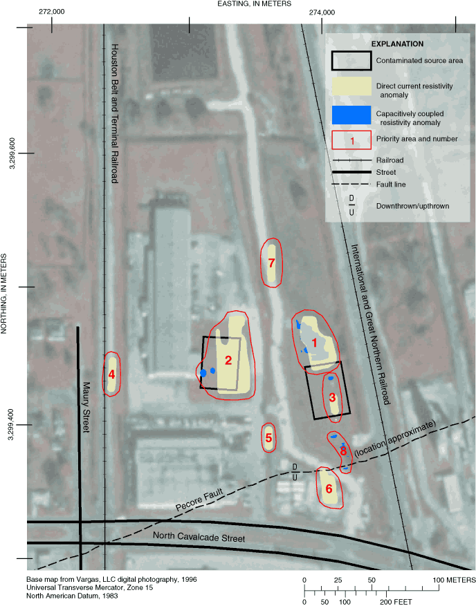
Priority area 1, which is partially within the northern part of the eastern contaminated source area, contains resistive anomalies that were identified using both 2D resistivity methods. Because resistive anomalies occurring in this area were verified with both methods, the area is located near the eastern contaminated source area, and the anomalies were identified in the inversion results of multiple survey lines for each technique, the resistive anomalies in this area received the highest priority. The inversion results of both 2D resistivity methods were used to identify resistive anomalies in priority area 2. The 2D resistivity survey of the western contaminated source area did not contain overlapping datasets that could be used for verification of the results; however, the inversion results of both methods were used to identify resistive anomalies occurring in multiple lines of the DC resistivity and, to a lesser extent, in two lines of the CC resistivity inversion results. Because the occurrences of resistive anomalies in this area were not verified by both methods, it received a lower priority, priority 2. Three anomalies were combined to form priority area 3. The three anomalies were not confirmed by both methods but they are located within or near the eastern contaminated source area. The resistive anomalies identified in areas 4 and 5 are from the inversion results of DC resistivity lines 2 and 3, respectively. Because only DC resistivity data were collected along these lines, they received a lower priority; however, they were higher in priority than 6 and 7 because they were not as close to gravel roads, gravel parking areas, or buildings. Resistive anomalies identified in priority area 8 occurred in only the inversion results of the CC resistivity survey, but the anomalies were not identified in the inversion results of the DC resistivity survey that was conducted in the same area.
The interpreted DC resistivity data allowed subsurface stratigraphy to be extrapolated between existing boreholes. The interpretations of the DC resistivity data also were used to determine the depth and extent of resistive anomalies and the stratigraphic unit or units in which they were situated. The interpretations of each line were evaluated to provide a brief description of interpreted subsurface features for each line. These descriptions were compiled in appendix 1, briefly listing general characteristics of strata I and II, stratum III, stratum IV, Pecore Fault, anomalies, priority areas, and any additional comments concerning interpreted subsurface features along each line. The results of inverse models, forward models, and interpretations from the 2D resistivity investigation and the compilation of these results (fig. 11 and app. 1) provide an improved understanding of lithologies that can influence the migration of contaminants and the possible extent and depth of creosote contamination at the North Cavalcade Street site.
The North Cavalcade Street site was first developed for wood treating by the Houston Creosoting Co., Inc. in 1946. The capabilities of the North Cavalcade Street site were increased in 1955 by adding pentachlorophenol wood preservation services and other support facilities, such as creosote ponds, pentachlorophenol and creosote storage structures, various tanks, lumber sheds, a treatment facility, and other buildings. By 1961, the property was closed. To protect public health and welfare and the environment from release or threatened releases of hazardous substances, the U.S. Environmental Protection Agency (USEPA) proposed that the North Cavalcade Street site be added to the National Priorities List on October 5, 1984. A remedial investigation conducted between September 1985 and November 1987 determined the locations of two contaminated source areas and a normal fault.
The record of decision released by the USEPA in 1988 required onsite biological treatment of soils containing carcinogenic polyaromatic hydrocarbons and ground water to be extracted and treated until all non-aqueous phase liquids were completely removed. However, since the first five-year review of the Record of Decision (July 1998), additional site characterization has confirmed that the dense non-aqueous phase liquid (DNAPL) extends to a deeper interbedded sand aquifer. Typically additional environmental site characterization used to determine depth and extent of DNAPL's and the lithologies in which they are contained has been through exploratory drilling. The accuracy of this method is dependent on the number of sample points or borings and the ability to interpolate between these sample points. Interpolation between sample points may be poorly constrained and lead to an inaccurate site characterization. An alternative approach is to combine surface geophysical methods with a drilling program.
During August 2003, the U.S. Geological Survey, in cooperation with the U.S. Environmental Protection Agency, conducted a two-dimensional resistivity investigation to aid in the North Cavalcade Street site characterization. The capacitively coupled (CC) resistivity method was used as a reconnaissance tool to locate geophysical anomalies that could be associated with possible areas of creosote contamination. The inversion results of the CC resistivity survey identified resistive anomalies in the subsurface near the eastern and western contaminated source areas. Based on the locations of anomalies found in the inversion results of the CC resistivity data, a direct-current (DC) resistivity survey near the CC resistivity survey confirmed the occurrence of most subsurface resistive anomalies.
Forward modeling was used as an interpretative tool relating the subsurface distribution of resistivity from four selected DC resistivity lines to known, assumed, and hypothetical information. Forward models were used to produce synthetic apparent resistivity datasets that were processed similarly to the field data. The forward models were refined until inversion results of the synthetic resistivity data and the field resistivity data approximately matched. The final forward models were used as an estimate of the true resistivity structure for the field data.
The forward modeling results for lines 1, 2, 6, and 11 were used to relate strata identified in geologist logs to the subsurface distribution of resistivity. Forward modeling was also used to test assumptions of the location and displacement of strata near the Pecore Fault. Because ground truthing of the inversion results was not included in this study, the true resistivity structure (depth, thickness, extent, and resistivity) of resistive anomalies identified in the inversion results of lines 1, 2, 6, and 11 were hypothesized and evaluated using the iterative forward modeling process.
The forward models and their inversion results were used to interpret the depth, thickness, and extent of strata and resistive anomalies occurring along lines 1, 2, 6, and 11 and the displacement of strata resulting from faulting near the Pecore Fault along lines 1 and 6. Lines 3, 5, 7-9, and 12-15 were interpreted using the relation developed between the inverted model datasets and the inverted field datasets for lines 1, 2, 6, and 11. Eight priority areas of resistivity anomalies were identified for evaluation in future studies. The results of inverse models, forward models, and interpretations from the 2D resistivity investigation and the compilation of these results provide an improved understanding of lithologies that can influence the migration of contaminants and the possible extent and depth of creosote contamination at the North Cavalcade Street site.
American Society for Testing and Materials, 1999, Standard guide for selecting surface geophysical methods in Annual book of ASTM standards: West Conshohocken, Pennsylvania, American Society of Testing and Materials, v. 04.08, p. 6429-6499.
Baker, G.S., 2003, Electrical resistivity 2D inversion tutorial: accessed July 16, 2004, at URL http://www.geology.buffalo.edu/courses/gly521/geophysics/2003_S01_ERInvertReport.pdf
CH2M Hill, 2003, Second five year review report for North Cavalcade Street, Houston, Harris County, Texas for USEPA Region 6: CH2M Hill, Work Assignment No. 948-FRFE-06ZZ, 29 p.
Camp Dresser & McGee Inc. (CMD), 1987, Remedial investigation report for North Cavalcade Street site, Houston, Texas for USEPA Region 6: Camp Dresser & McGee Inc., Document Control No. 141-RI1-RT-FGJC-1.
Degnan, J.R., Moore, R.B., and Mack, T.J., 2001, Geophysical investigations of well fields to characterize fractured-bedrock aquifers in southern New Hampshire: U.S. Geological Survey Water-Resources Investigations Report 01-4183, 54 p.
Geometrics, Inc., 2002, Magmap 2000 User Guide—24891-01 Revision G: Geometrics, Inc., 228 p., accessed September 12, 2005 at http://www.geometrics.com/Downloads/MagDnForm/MagDown/magdown.html
Geometrics, Inc., 2004, OhmMapper-Resistivity Mapping: accessed July16, 2004, at URL ftp://geom.geometrics.com/pub/imagem/DataSheets/OhmMapBro.pdf
Guy, E.D., Daniels, J.J., Holt, J., Radzevicius, S.J., and Vendl, M.A., 2000, Electromagnetic induction and GPR measurements for creosote contamination investigation: Journal of Environmental Engineering Geologist, v. 5, no. 2, p. 11-29.
Loke, M.H., 2002a, Tutorial—2-D and 3-D electrical imaging surveys—M.H. Loke, 110 p.: accessed December 1, 2003, at URL http://www.geoelectrical.com/download.html
Loke, M.H., 2002b, RES2DMOD version 3.01—Rapid 2D resistivity forward modeling using the finite-difference and finite element methods: accessed October 1, 2003, at URL http://www.geoelectrical.com/download.html
Loke, M.H., 2004a, RES2DINV version 3.54—Rapid 2D resistivity and IP inversion using the least-squares method: Geoelectrical Imaging 2-D and 3-D—Geotomo Software, 130 p. accessed September 12, 2005, at URL http://www.geoelectrical.com/download.html
Loke, M.H., 2004b, RES3DINV version 2.14—Rapid 3D resistivity and IP inversion using the least-squares method: Penang, Malaysia, Geotomo Software, 70 p.
Powers, C.J., Wilson, Joanna, Haeni, F.P., and Johnson, C.D., 1999, Surface-geophysical characterization of the University of Connecticut landfill, Storrs, Connecticut: U.S. Geological Survey Water-Resources Investigations Report 99-4211, 34 p.
Stanton, G. P., Kress, W.H., Hobza, C. M., and Czarneci, J.B., 2003, Possible extent and depth of salt contamination in ground water using geophysical techniques, Red River aluminum site, Stamps, Arkansas, April 2003: U.S. Geological Survey Water-Resources Investigations Report 03-4292, 28 p.
U.S. Army Corps of Engineers, 1995, Geophysical exploration for engineering and environmental investigations: Engineering Manual 1110-1-1802, chap. 4, 57 p.
U.S. Environmental Protection Agency, 2003, Site status summaries-Texas—North Cavalcade Street: accessed November 17, 2004, at URL http://www.epa.gov/earth1r6/6sf/pdffiles/0602956.pdf
[m, meters; ~, approximately; <, less than; >, greater than; CSA, contaminated source area; N, north; S, south; E, east; W, west; n/a, not applicable]
| Section | Average surface elevation | Strata I and II | Stratum III | Stratum IV | Pecore Fault | Anomalies | Priority area + | Comments |
|---|---|---|---|---|---|---|---|---|
| Fig. 9C, line 1 | 14.5 m | 14.5 to 9.5 m in elevation <1 to 4.5 m thick | 13.5 to 4.5 m in elevation 2.0 to 8.0 m thick | 12.0 to < 3 m in elevation* | 5 m upthrown to S | 14.5 to 13.5 m in elevation ~ 1 m thick ~ 20 m wide N to S near eastern CSA | 1 | Some shallow sand channels on lower clay |
| Fig. 9F, line 2 | 15.0 m | 15 to 5 m in elevation < 1 to 10.0 m thick | 15 to -1 m in elevation < 1 to 10.0 m thick | 10.0 to < -45 m in elevation* | not present | 15 to 12 m in elevation 1 to 3 m thick ~ 38 m wide N to S | 4 | Unknown unit appears below -40 m in elevation to the N |
| Fig. 9I, line 6 | 14.8 m | 14.8 to 11.5 m in elevation <1 to 3.5 m thick | 14.8 to 5.0 m in elevation 2.0 to 8.0 m thick | 10.5 to < -3 m in elevation* | 3 m upthrown to S | N of eastern CSA: 14.8 to 12.3 m in elevation 2.5 m thick ~ 30 m wide N to S | 1 | Two separate anomalies |
| S of Pecore Fault: 14.8 to 11 m in elevation 0.5 to ~ 4 m thick ~ 15 m wide N to S | 6 | |||||||
| Fig. 9L, line 11 | 14.7 m | 14.0 to 11.0 m in elevation 2.0 to 3.0 m thick | 14.7 to 14.0 m and 11.5 to 58.0 m in elevation <1 m and 2.0 to 5.0 m thick | 8.0 to < 4 m in elevation* | not present | 14.8 to 12.8 m in elevation < 1 to 2 m thick | 2 | Anomaly extends along most of the section N-S |
| Fig. 10A, line 3 | 14.7 m | 14.7 to 12.5 m in elevation < 1 to 2.0 m thick | 14.7 to 13.0 m and 14.0 to 1.0 m in elevation < 1.5 m and 1.0 to 12.0 m thick | 12.0 to < -5 m in elevation* | 5 m upthrown to S | 14.7 to 12.5 m in elevation < 1.0 to 2.0 m thick < 25 m wide N to S | 5 and 7 | Three anomalies N of Pecore Fault, fine sand at surface, deep channels in lower clay up to 10 m in depth |
| Fig. 10B, line 5 | 14.8 m | 14.8 to 11.0 m in elevation < 1 to 3.0 m thick | 14.8 to 4.0 m in elevation 2.0 to 8.0 m thick | 10.0 to < -3 m in elevation* | ~5 m upthrown to S | S or Pecore Fault: 14.8 to 10.5 m in elevation ~ 4 m in thick ~15 m wide N to S | 6 | Some 1 to 5 m fine sand channels on top of lower clay unit |
| N of eastern CSA: 14.8 to 13.0 m in elevation ~1.5 m thick ~ 10 m wide N to S | 1 | |||||||
| Fig. 10C, line 7 | 14.8 m | 14.8 to 7.0 m in elevation <1 to 7.0 m thick | 14.8 to 3.0 m in elevation 1 to 7.0 m thick | 12.0 to < -3 m in elevation* | 6m upthrown to S; sand thinnest to S | N of eastern CSA: 14.8 to 11.0 m in elevation 1.0 to 3.0 m thick ~ 25 m wide N to S | 1 | Two separate anomalies, southern anomaly small |
| S of Pecore Fault 14.8 to 14.0 m in elevation < 1 m thick < 4 m wide | 6 | |||||||
| Fig. 10D, line 8 | 14.7 m | 14.7 to 12.0 m in elevation < 1 to 2.5 m thick | 14.7 to 3.0 m in elevation < 1 to 9.0 m thick | 12.5 to < -3 m in elevation* | ~4 m upthrown to S | N of eastern CSA 14.7 to 6.0 m in elevation 3.0 to 8.0 m thick ~ 18 m wide N to S | 1 | Northern anomaly extends to top of lower clay unit |
| Within eastern CSA 14.7 to 10 m in elevation ~ 5 m thick ~ 15 m wide | 3 | |||||||
| Fig. 10E, line 9 | 14.6 m | 14.6 to 13.0 m in elevation < 1 to 1.5 m thick | 14.6 to 5.0 m in elevation 4.5 to 8.0 m thick | 11.0 m to < -3 m in elevation * | ~ 5m upthrown to S | none observed | n/a | Thin to discontinuous upper clay |
| Fig. 10F, line 12 | 14.7 m | 14.7 to 10.0 m in elevation 3.0 to 4.5 m thick | 11.5 to 7.0 m in elevation 2.0 to 4.5 m thick | 9.0 to < 4 m in elevation* | not present | 14.7 to 13.0 m in elevation < 1 to 1.5 m thick | 2 | Anomalies along entire length of section, N-S, varying thickness |
| Fig. 10G, line 13 | 14.8 m | 14.8 to 9.0 m in elevation 2.0 to 5.0 m thick | 12.0 to 7.0 m in elevation 2.0 to 5.0 m thick | 8.0 to < 4 m in elevation* | not present | 14.8 to 13.0 m in elevation <1 to 1.5 m thick | 2 | Anomalies along entire length of section, N-S, varying thickness |
| Fig. 10H, line 14 | 14.8 m | 14.8 to 10.0 m in elevation < 1 to 5.0 m thick | 14.8 to 13.5 m and 13.0 to 7.5 m in elevation < 1 to 1.5 m and 1.0 to 4.0 m thick | 9.0 to < 6 m in elevation* | not present | 14.8 to 13.0 m in elevation < 1 to 1.5 m thick | 2 | Upper fine sand in N part of site, several anomalies in western CSA |
| Fig. 10I, line 15 | 14.9 m | 13.0 to 10.5 m in elevation | 14.9 to 12 m and 13.0 to < 6 m in elevation | 9.0 to < 6 m in elevation* | not present | 14.9 to 13.0 m in elevation | 2 | Fine sand separated by sandy clay/clayey sand, continuous anomaly in western CSA with some small anomalies extending N |
* Layer extends below the depth of investigation. Thickness cannot be estimated.
+ Priority area 8 includes resistive anomalies from capacitively coupled resistivity results. Anomalies were unable to be confirmed by direct-current resistivity results; therefore, priority area 8 is not included in this summary.
Document Accessibility: Adobe Systems Incorporated has information about PDFs and the visually impaired. This information provides tools to help make PDF files accessible. These tools convert Adobe PDF documents into HTML or ASCII text, which then can be read by a number of common screen-reading programs that synthesize text as audible speech. In addition, an accessible version of Acrobat Reader 6.0, which contains support for screen readers, is available. These tools and the accessible reader may be obtained free from Adobe at Adobe Access.
| AccessibilityFOIAPrivacyPolicies and Notices | |
 |
|